Pranjal's Blog

Proud Fast.ai student

Home Atom Feed home RSS Feed Sitemap Offline CV About

All posts in one long list

A deeper understanding of NNets (Part 4) - AutoEncoders

Feb 11, 2018 on AutoEncoders Deep Learning Neural Network ML AI

Review

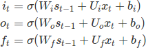
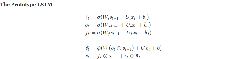
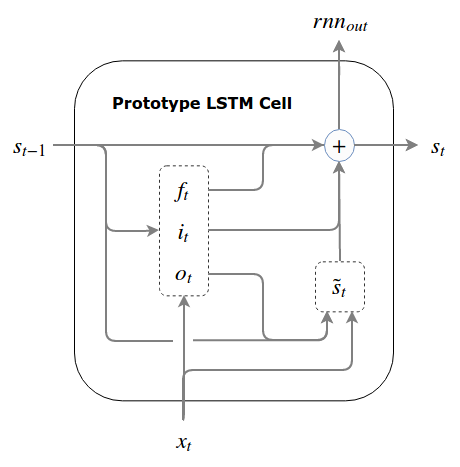
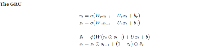
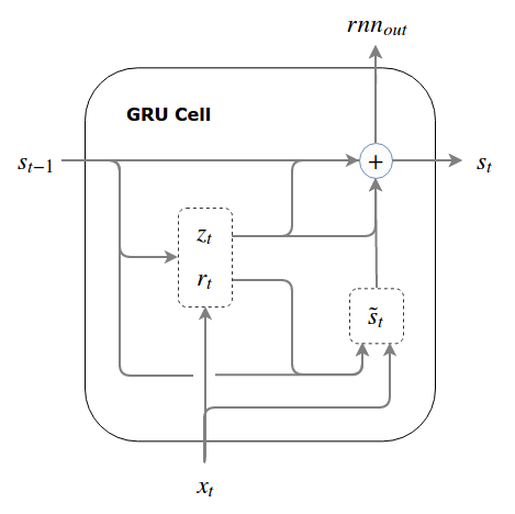
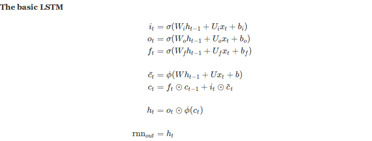
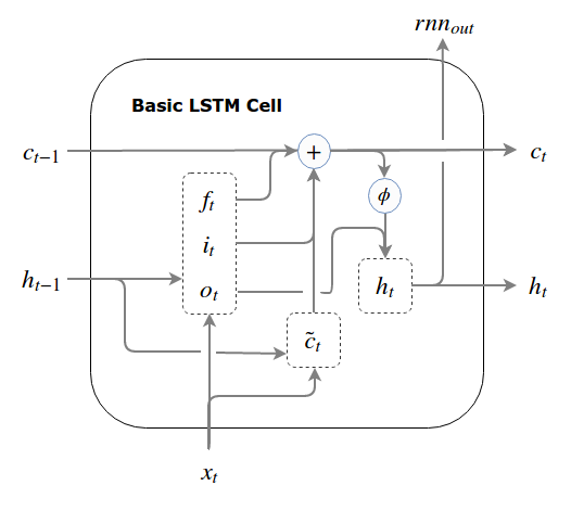
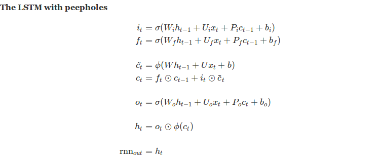
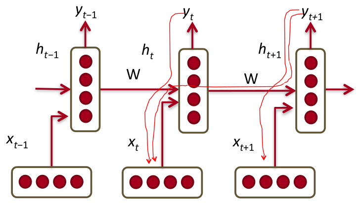
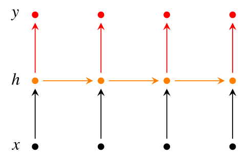
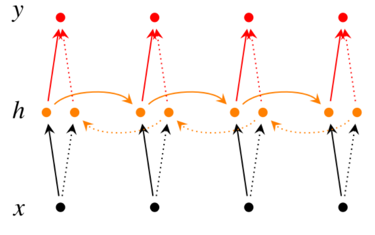
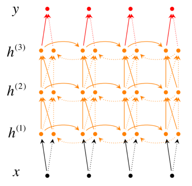
In the last post we discussed about LSTMs and GRUs, diving deeper into their existence and importance over regular RNNs. Though they are a bit complex, yet they belong to a supervised learning realm which feels intuitive to a large extent when training machine learning models. In next few posts, we will be looking at methods primarily used for deep leaning but with a unsupervised approach.

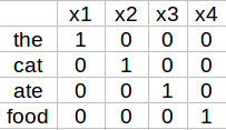
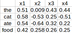
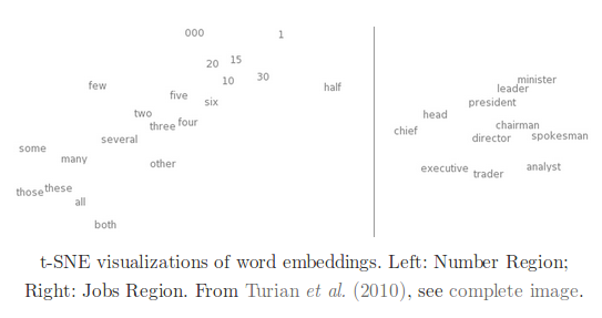
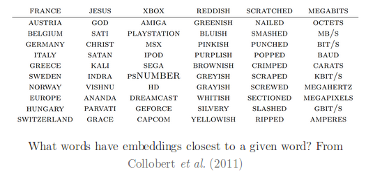
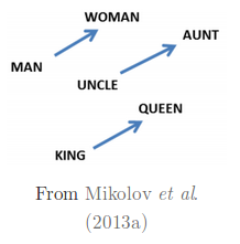
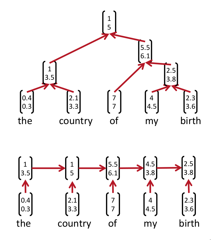
To start with, we will focus on the benefits of latent representation of data and learning methods to find them. As we discussed earlier in RNNs, embeddings are latent representation of text, similarly, we can find latent representation of images or any other format of unstructured data. But rather than finding a higher dimensional vector representation like embeddings, now we want to focus on learning lower dimensional representation of the data. In this post we will discuss AutoEncoders in great details and set the stage for GANs, RBMs and other NNets which utilize the same concept of information extraction into a lower dimensional space.

AutoEncoders

As the name suggests, AutoEncoders are encoding information without any prior knowledge about the type or distribution of information (technically making them automatic) and hence the name AutoEncoders (AE here on).

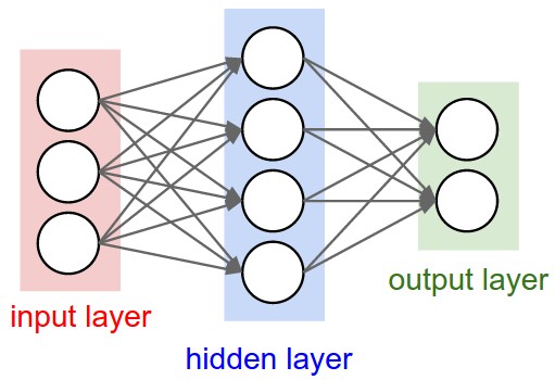
An AE is primarily composed of three parts, an input layer, a hidden layer and a decoding layer. The purpose of this network is to learn the input and recreate it after understanding it! You may come across standard definition saying an AE recreates the input and they are perfectly OK, but then it creates the doubt that is it learning an identity function? meaning is it only replicating the input. Which is not the case and hence the added part to the definition “after understanding it”.

Lets have a close look at the architecture

Autoencoder (Img Src : http://ufldl.stanford.edu)

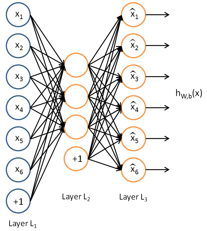
The AE is trying to learn hW,b(x)≈x, which in essence is equivalent to approximating an identity function but not equal. The difference comes from the design of architecture where we constrain the count of hidden nodes after the input layer. This forces the network to learn weights with which it can still contain the same amount of information but in a lower dimensionality and hence an encoded state which is not an identity state.

However, it is also possible to have higher count of hidden nodes and still find the same amount of information, this is achieved by (as you might have guessed) adding an activation function and limiting the total count of activated nodes to a very low number. This fundamental technique is forcefully introducing sparsity in the network allowing us to achieve the same low dimensional representation. The constant number enforcing the fraction of possible activation is the “sparsity parameter”, now lets dive a little deeper into the math of it.

You can recall that an activation function a(say sigmoid) on an input x gives the output p which is between 0 to 1. This activation acts as a on/off switch for any node in the network (We can achieve the same with tanh as well by defining -1 and 1 as the two states). Now comes the most tricky and fundamental part, if we set the sparsity parameter as p' and define p = a(x), what we are trying to optimize for is p = p'.

Think about it, if the activated output and the sparsity constraints is equal, the output from the activation is 1) densely packed or lower dimensionally encoded (we usually set the sparsity parameter close to 0, for examples 0.05) and 2) it still learned to represent the input x using the network and the activations. So the optimized state directly states “the leaned representation in hidden state is a lower dimensional representation of the input aka the CODE of the AE”. Just to validate our learning, we add a decoding part to the network so that the network can now use the CODE to recreate what it started with and utilize back-propagation to optimize iteratively.

After successfully reducing the loss or finding the best possible CODE, the autoencoder has learned the latent representation of the input data, we can alternatively say, it has learned the distribution of the input data.

NOTE: The optimum state where p' = p is also called the minimum of KL divergence. You can read about it in great details on the web, I suggest this video.

Visualizing an AutoEncoder (Refreshing CNNs)

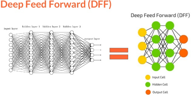
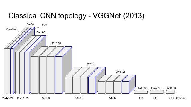
The CODE state of an AE is quite similar to the convolutions learned by a CNN, the difference is, for CNNs the convolutions points to a class(indirectly) and different classes helps build different layers of convolutions as opposed to AEs which try to learn the distribution of the input data so that it can recreate similar new outputs from the learned distribution. For example, the imagenet dataset with 1000 classes help learn edge detection, geometrical shapes, gradients and then faces or more complex/convoluted features from the data, but it only does so to be able to find the boundary condition so that later it can do the classification.

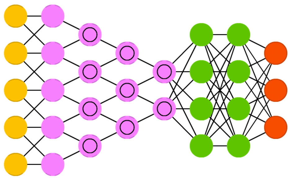
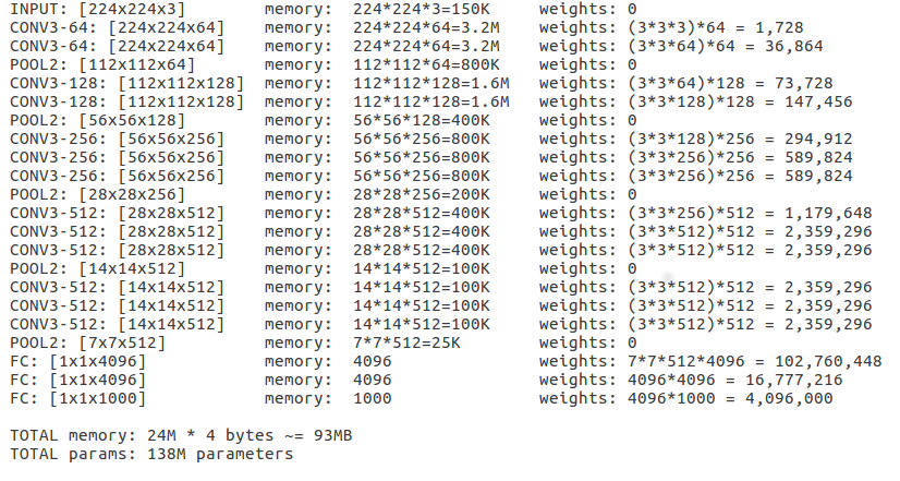
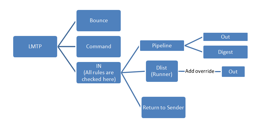
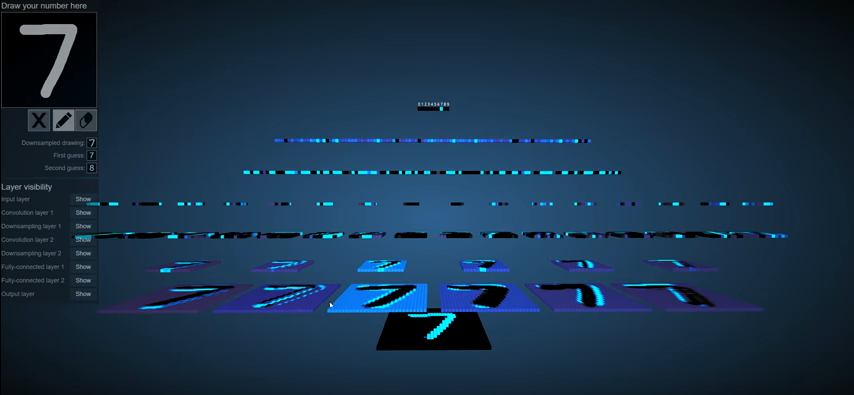
If we look at the rotated view of a CNN forward pass on an image, it looks like a tree with child nodes equal to learned convolutions. While testing an image, it parses the image through this tree structure to gives the highest probability for a class.

NOTE: Fundamentally the encoder half of an AutoEncoder acts as a recognition model and is similar to a CNN, the utilization of the learned representation for AEs and convolutions of CNNs sets them apart.

Tree like view of CNNs

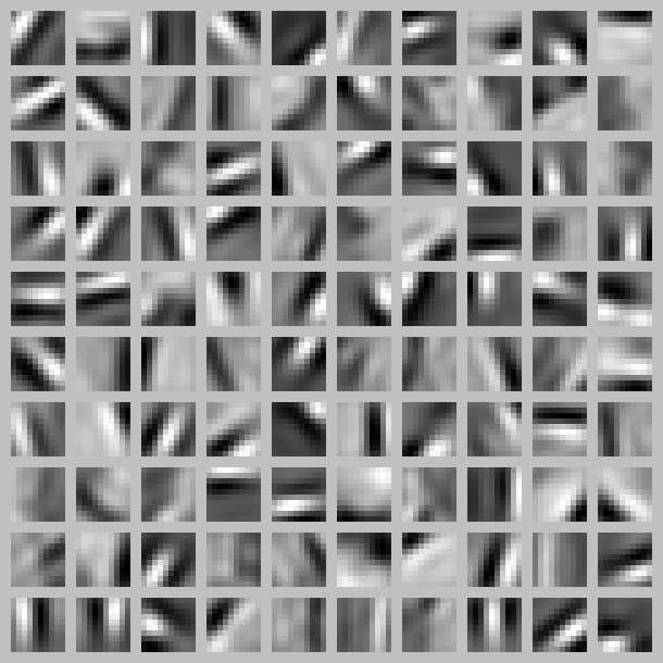
If we look at the CODE for an AE trained on a similar dataset, it looks like an edge detector, but additionally it learned the relative position or better to say, the distribution of the placement of learned edges from the training dataset.

Learned CODE for AutoEncoder

PS: I’m unsure if we can de-couple the convolutions from a CNN and use them as the CODE state with a pre-trained decoder to generate new images/outputs.

Types of AutoEncoders

There are various types of AutoEncoders out there but we will focus on the 4 types clearly mentioned in wikipedia. 1) Denoising AutoEncoder 2) Sparse AutoEncoder 3) Variational AutoEncoder and 4) Contractive AutoEncoder

Denoising AutoEncoder: The idea is to force the autoencoder to de-noise the data and extract the CODE, to do that, we intentionally add noise with the input data. This technique is an example of good representation which is defined as ‘a representation that can be obtained robustly from a corrupted input and that will be useful for recovering the corresponding clean input’. The only difference while running the code for a denoising autoencoder vs a vanilla autoencoder is passing the noised input rather than the original input and still comparing with the original input.
Sparse AutoEncoder: We discussed this approach while defining the AutoEncoders.
Contractive AutoEncoders: They are simply regularized vanilla autoencoders allowing the models to be more robust against slight variations in the input.
Variational AutoEncoders (VAE): This approach differs in the learning process, a vanilla autoencoder learns the latent representation(CODE) without any prior assumption or belief, whereas VAE assumes that the data is generated by a directed graphical model and that the encoder is learning an approximation to the posterior distribution. I understand that this doesn’t make much sense and for the enormosity and depth of VAE, I will dedicate the next post for a deep dive on VAE and it will also help bring in comparison with GANs. Stay tuned for VAEs…

Conclusion

AutoEncoders are effective way of finding specific latent representation of the training data and there are various implementations and their stacked versions to utilize the best of autoencoders. The encoder is responsible for creating the best patent representation and the decoder is responsible to recreate the input using the learned representation. This makes the decoder half of the AutoEncoder a generative model like GANs. We will look at various generative modeling techniques in the coming posts.

Thank you for reading, I hope it helped

A deeper understanding of NNets (Part 3) - LSTM and GRU

Nov 19, 2017 on RNN LSTM Deep Learning ML AI

Review

In the last post we talked about RNNs in brief and discussed about statefullness and recurrence. We also looked at vanishing/exploding gradients problem and understood how bi-directional RNNs work. To solve for the vanishing gradients problem, researchers developed on an already existing idea and improved upon capturing the long-term dependencies by introducing the LSTM Networks. In the following section, we will deep dive into LSTM and understand how it led to the development or GRUs or Gated Recurrent Units.

LSTM

Vanishing Sensitivity of vanilla RNNS is proven mathematically and comprises two major factors 1. Weight Initialization 2. Back-propagation

Weight Initialization is not a direct solution to avoid vanishing gradients but it helps avoiding any immediate problems. Back-propagation on the other hand is the primary cause of vanishing gradients, this problem becomes more escalated when back propagation and simultaneous forward passes are done to compute error gradients with respects to weights at each time step, read real-time recurrent learning (RTRL) for more info. So it seems a good idea to truncate the back propagation, but knowing when to truncate the back propagation is important because we need to update the weights accordingly allowing the model to progress. Therefore, the solution to vanishing gradients is two parts, knowing how often to truncate the back propagation and how often to update the model.

After having solved for vanishing gradients, researchers also wanted to solve for the information morphology problem posed by the vanilla RNNs. In simple words, the information contained in a prior state gets embedded over and over due to non-linearities and is not the best usable state of information in its current state. In essence, the original usable information is lost in the morphed information.

The originality of information can be preserved and this was proposed by the landmark paper of Hocreiter and Schmidhuber (1997). They asked: “how can we achieve constant error flow through a single unit with a single connection to itself [i.e., a single piece of isolated information]?”

The answer, quite simply, is to avoid information morphing: changes to the state of an LSTM are explicitly written in, by an explicit addition or subtraction, so that each element of the state stays constant without outside interference: “the unit’s activation has to remain constant which is ensured by using the identity function”. Hocreiter and Schmidhuber observed that simple addition or subtraction of information at each state may keep the state isolated but at the same time, the addition and subtraction may cancel out or worse, they may complicate the states with only parts of information preserved which gets hard to recover.

Hochreiter and Schmidhuber recognized this problem, splitting it into several subproblems, which they termed “input weight conflict”, “output weight conflict”, the “abuse problem”, and “internal state drift”. The LSTM architecture was carefully designed in order to overcome these problems, starting with the idea of selectivity.

As per the LSTM literature, there are 3 things a LSTM should selectively decide, “what to write, what to read and what to forget”. The most fundamental and mathematical way of maintaining selectivity is gates, we call these gates the read, write and forget gates. Our three gates at time step t are denoted i(t), the input gate (for writing), o(t), the output gate (for reading) and f(t), the forget gate (for remembering!).

Here are the mathematical definitions of the gates (notice the similarities):

Equations governing LSTM.

With all the gates defined, we now develop a LSTM prototype by defining the required behavior. To write a candidate state s(t), we follow a simple rule of thumb.

Take the inputs using the write gate
Calculate the output using the read gate (output is reading the input information so you can remember that it uses the read gate and not the input)
Combine the output with relevant prior information, for keeping relevant information we use the forget gate with prior state.

Equations governing LSTM.

Below is a pictorial view of above equations with arrows pointing to flow of data within the LSTM cell.

A LSTM cell.

In theory, this prototype should work but turns out it doesn’t. It happens because, even after well thought initializations and write and forget gates, the coordination between these gates in early stage of training gets tricky and very often it becomes large and chaotic at write step. For more details, refer to “internal state drift” problem, further, an empirical demonstration of this can be found in Greff et al. (2015), which covers 8 variants of LSTMs.

The solution to above problem is bounding the state to prevent it from becoming chaotic or blowing up. There are 3 variants of LSTM which uses this solution 1. Normalized LSTM, GRU and Pseudo LSTM. We will focus mainly on the GRU for this post but feel free to dive deeper into the other variants.

GRUs

We impose a hard bound on the state by explicitly binding the write and forget gate. In other words, instead of doing selective writes and selective forgets, we define forget as 1 minus write gate. So whatever is not written is forgotten. In the GRU terminology, the forget gate is renamed as update gate or z(t) and it essentially means “do-not-update”. So an element wise update on prior state would tell what not to update and 1 - z(t) actually updates the state behaving as the new write gate.

Equations governing GRU.

Below is a pictorial view of above equations with arrows pointing to flow of data within the GRU cell.

A GRU cell.

Note the difference between reads and writes: If we choose not to read from a unit, it cannot affect any element of our state and our read decision impacts the entire state. If we choose not to write to a unit, that impacts only that single element of our state. This does not mean the impact of selective reads is more significant than the impact of selective writes: reads are summed together and squashed by a non-linearity, whereas writes are absolute, so that the impact of a read decision is broad but shallow, and the impact of a write decision is narrow but deep.

You might still be wondering that the LSTM cell we talked about doesn’t quiet look like the Basic LSTM cell available all over Internet and you are right. The reason is we didn’t define the Basic LSTM cell above, we defined a prototype cell we sequentially answered all the problems faced with vanilla RNNs. We will now move forward to define the Basic LSTM cell.

Basic LSTM cell

As we discussed above, read comes after write because the cell writes the input to memory and then reads the output during calculation followed by finally applying the forget gate and update the cell. Here we loosely used the term memory which plays an important role in the construct of basic LSTM cell. The Basic LSTM cell requires a small change from our prototype, we will now input 2 priors to a cell, namely, previous state s(t) now renamed as c(t) and a shadow/hidden state h(t). Hidden state is nothing but a gated previous state and additionally the previous also flows in the cell. The output of this a an updated current state along with a hidden state which is a gated current state.

If we think carefully, the basic LSTM is taking the previous state in 2 forms, directly and gated (other than the external input)and producing current state in 2 forms, directly updated ans its gated version. The primary reason of introducing all this complexity and the hidden states is the “write then read order”. We need to read the previous state in order to create a current candidate write. But if, creating the current candidate write, comes before the read operation inside our cell, we can’t do that unless we pass a pre-gated “previous state”, which makes hidden states compulsory. The write-then-read order thus forces the LSTM to pass a hidden state from cell to cell.

Basic LSTM equations updated with respect to the memory cell view.

Below is a pictorial view of above equations with arrows pointing to flow of data within the Basic LSTM cell.

A Basic LSTM cell, as available across Deep Learning Libraries.

Though this implementation of LSTM is stable and scales well, the unmodified previous state input is sometimes re-wired to flow into the gates calculation giving birth to LSTM with peepholes, which is simply another variant of LSTM. The primary difference with peephole LSTM is that the updated current state is used for output via read gate as opposed to the prior state read by the Basic LSTM cell.

Governing equations of LSTM with peepholes.

Conclusion

LSTM and its variants solved the fundamental (information morphing) and technical (vanishing gradients) problems associated with RNNs and thus gained popularity. The ideology associated with LSTM and its variants also allowed researchers to implement a similar thought process of selectivity while reading and writing information. This ideology paved way for the Residual Networks or ResNet combined with very deep (upto 100s of layers) architecture. This network won the ImageNet 2015 competition.

The content of this post might get confusing with a visual depiction and thanks to deepsystems.ai you can watch the video for a better understanding. Their video and quoted text of this post is inspired by R2RT’s blog post: Written Memories: Understanding, Deriving and Extending the LSTM.

In the next post, we will look at Auto Encoders in detail and also explore their utility in modern architectures.

Thank you for reading, I hope it helped

A deeper understanding of NNets (Part 2) - RNNs

Jul 27, 2017 on RNN LSTM Deep Learning ML AI

Review

Last week we talked about a very particular type of NNet called Convolutional Neural Network. We can definitely dive deeper into Conv Nets but the essence of the topology was broadly covered in the previous post. We will revisit the Conv Nets after we have covered all the topologies, as discussed in the previous post.

Week 2

The architecture for this week is Recurrent Neural Network or RNN. The key difference between a RNN and any Feed Forward Normal/Deep Network is the recurrence or cyclic nature of this architecture. It sounds vague in the first go but lets unroll this architecture to understand it better. We will also be discussing two special cases of RNN namely LSTM and GRU in the next post.

Why do we need RNNs? Lets find out.

Lets take a use-case of RNN, Natural Language Processing (NLP), traditional NLP techniques used statistical methods and rule-based approach to define a language model. Language models computes a probability for a sequence of words: P(w1, w2, ….. wn) which is useful in machine translation and word prediction.

These traditional models have 3 major challenges:

Probability was usually conditioned over n previous words.
An incorrect but necessary Markov assumption.

To estimate any probability they had to compute n-grams.

Computation of so many n-grams has HUGE RAM requirements, which gets practically impossible after a point. Also, above models relied on hand engineered linguistic features to deliver state-of-the-art performance.

RNNs solve the above problems by using a simple solution called “statefulness” and “recurrence”. Deep Learning allows RNN to remember or forget things based on few logical values, as we will see later, and perform cyclic operations within the network to achieve better results. Before we start exploring how all this happens, lets first understand a crucial input that goes into RNN, Word Embeddings.

Word Embeddings

Introduced by Bengio, et al. more than a decade ago, these are powerful representation of simple words. For example, the sentence “the cat ate the food” is the input to a language model, now we need to convert this sentence into numbers for the network to process it. The simplest way is to form One-Hot vectors of vocabulary.

One Hot Encoding

Although this looks simple and gets the job done, think of a scenario where our vocabulary has a Billion words, then we would need 1Bx1B matrix, which is extremely sparse and GIGANTIC in size. To solve this problem, we can develop word embeddings which are dense representation of the word along with its meaning, context, placement in sentence and much more. More technically, word embeddings are a parameterized function mapping in some language to high-dimensionality.

Word Embeddings

These vectors are dense and allow for more information to be captured for every word, though the meaning of these vectors are a mystery, yet they are more likely to explain a word with better meaning given a large vocabulary set and the dimensionality of these embeddings can be as high as 200 to 500. We can set these embeddings as random and train on our corpus or we can choose transfer learning and utilize pre-trained word representation like Word2Vec and Glove. One thing we can do to understand these embeddings is use a dimensionality reduction technique called t-SNE which helps in visualizing high dimensional data.

It seems logical for a network to have similar vectors for similar words and if we cluster them after t-SNE the results are fairly intuitive.

It gets magical when we see analogies encoded as difference in these word vectors, meaning a euclidean distance between words is analogical to their actual meaning set in the language.

Word Embeddings forming analogies.

It is safe to assume that if a network is trained over a huge corpus, word embeddings obtained can provide country:language, state/nation:capital, job:role and far more sophisticated relationships. Word embeddings also allow bilingual word connections and entity to image mapping but we will focus on RNNs for this part.

Recurrent Neural Networks

A simple RNN takes a word embedding as input, perform some matrix operations, achieves an interim output called hidden state and then using an activation and previous hidden state it outputs the prediction. Lets assume its a word prediction model and the current output from the model is the most probable word after the first input, so the output for word ‘cat’ should be ‘ate’.

Single layer of RNN.

Repeating several such layers makes a RNN recurrent as it visits the information obtained till previous iteration to utilize it in current iteration. There are two ways to look at it, I personally prefer the unfolded depiction of RNNs but people use a cyclic notation as well which seems intuitive.

Unfolded view of RNN. Cyclic layer RNN

Cyclic view of RNN.

Elaborating on our previous example, the word embedding of cat (lets say we{cat}) takes input from we{the} to predict “ate”, in the next step, we{ate} takes input as combined information from the previous hidden state and account for both we{the} and we{cat} directly to predict “the”. The final iteration will incorporate we{the} with hidden state from previous iteration accounting for we{the}, we{cat}, we{ate} and re-appearance of we{the} to predict “food”. In principle, the network understood the underlying structure of sentence.

Exploding/vanishing gradients

The major problem with RNNs is something called vanishing gradient, since it utilizes the previous hidden state to predict current output, it back-propagates through all hidden states and following the chain rule, the gradients multiply at each iteration finally becoming approximately zero after 7 to 8 words. This doesn’t allow the network to train as expected! Another variant of the same problem is exploding gradient which occurs when the weights of the hidden states are greater than 1, back-propagating leads to infinitely huge values. However there is a simple solution proposed by researchers to avoid exploding gradients which is simply capping the value of gradients to a max. So the only problem we need to deal with is vanishing gradients. Lets welcome the two most popular variant of a RNN, LSTM (Long-Short-Term-Memory) and GRU (Gated Recurrent Unit) networks, we will discuss them in detail in the upcoming post. But before discussing LSTMs and GRUs lets fancy ourselves with Bi-Directional RNNs.

Back propagation leading to vanishing gradients.

Bi-Directional RNNs

A simple RNN looks like the below diagram, however, if we choose to utilize ‘the next and the previous’ hidden states to predict current output then its called a Bi-Directional RNN. Going ‘deeper’ if we allow more than one hidden layers before our output then its called a Deep Bi-Directional RNN.

A simple RNN in a different view.

A Bi-Directional RNN.

A Deep Bi-Directional RNN.

How does recurrence helps? Is it same as Recursive Neural Networks?

As we discussed above, recurrence is simply using information from previous hidden state which in turn uses previous hidden state so on and so forth. In the “cyclic view” it is easier to understand the “re-occurrence” of referring back to all previous hidden state, which brings the name recurrence. However, we must not confuse it with Recursive Neural Networks which are TREE type RNNS. We can debate that recurrence and recursive indicate the same notion of matrix operations within a network but the structural implementation to utilize this notion of matrix operations to process information sequentially sets them apart. Below example clearly separates the “Recurrent” and “Recursive” neural networks.

Recursive vs. Recurrent Neural Network.

In theory, the recursive NNets require parser to form a tree structure but at the same time, a good parser will allow a tree structure capturing long distance context without a huge bias on the previous word. On the other hand recurrent NNets often capture too much of last word.

Statefulness of RNNs

RNNs can be stateful, which means that they can maintain states during training. As you might have guessed, these states are the hidden states which we saw earlier. The benefits of using stateful RNNs are smaller network sizes and/or lower training times. The disadvantage is that we are now responsible for training the network with a batch size that reflects the periodicity of the data, and resetting the state after each epoch. In addition, data should not be shuffled while training the network, since the order in which the data is presented is relevant for stateful networks.

RNNs by default are trained stateless and we need to explicitly tell the network to maintain states if we wish to use them. We will use this property while discussing LSTMs and GRUs in the next post.

Conclusion

RNNs are powerful NNets not only because they are great at NLP, but in general RNNs dominate in more general purpose tasks. You can read “The Unreasonable Effectiveness of Recurrent Neural Networks” by Andrej Karpathy here. It explains RNNs’ Turing-Complete ability and highlights the benefits of one/many to one/many network representation.

In the next post, we will look at LSTMs and GRUs in detail and also explore few LSTM variants.

Thank you for reading, I hope it helped

A deeper understanding of NNets (Part 1) - CNNs

Jul 20, 2017 on Machine Learning Deep Learning ML AI DL

Introduction

Deep Learning and AI were the buzz words for 2016; by the mid-2017, they have become more frequent and more confusing. So lets try and understand everything one at a time. We will look into the heart of Deep Learning i.e. Neural Networks (NNets). Most variants of NNets are hard to understand and the underlying architectural components make them all sound (theoretically) and look (graphically) the same.

Thanks to Fjodor van Veen from The Asimov Institute, we have a fair representation of the most popular variants of NNet architectures. Please refer to his blog. To improve our understanding of NNets, we will study and implement one architecture every week. Below are the architectures we will be discussing over the next few weeks.

Week 1

The architecture for this week is Convolutional Neural Network or CNN. But before starting CNN, we will first have a small deep dive into Perceptrons. NNet is a collection of several units/cells called perceptrons which are binary linear classifiers. Lets take a quick look to understand the same.

Inputs x1 and x2 are multiplied with their respective weights w1 and w2 and summed together using function f, therefore f = x1*w1 + x2*w2 + b(bias term, optionally added). Now this function f can be any other operation but for perceptrons its generally a summation. This function f is then evaluated through an activation which allows the desired classification. Sigmoid function is the most common activation function used for binary classification. For further details on perceptrons, I recommend this article.

Now if we stack multiple inputs and connect them using function f with multiple cells stacked in another layer, this forms multiple fully connected perceptrons, the output from these cells(Hidden layer) becomes input to the final cell which again uses function f and activation to derive final classification. This, as show below, is the simplest Neural Network.

The topologies or architectural variants of NNets are diverse because of a unique capability of NNets called “Universal Approximation function”. This in itself is a huge topic and is best covered by Michael Nielsen here. After reading this we can rely on the fact that NNet can behave as any function no matter how complex. Above mentioned NNets is also referred to as Feed Forward Neural Network or FFNN, since the flow of information is uni-directional and not cyclic. Now that we know the basics of perceptron and FFNN, we can imagine hundreds of inputs connected to several such hidden layer, would form a complex network popular called Deep Neural Network or Deep Feed Forward Network.

How exactly is a Deep Neural Network different from CNN? Let’s find out.

CNNs gained their popularity through competitions like ImageNet and more recently they are used for NLP and speech recognition as well. A critical point to remember is that many other variants like RNN, LSTM, GRU etc are based on a similar skeleton as that of CNNs but with some difference in architecture that makes them different. We will later discuss the differences in detail.

CNNs are formed using 3 types of layers namely “Convolution”, “Pooling” and “Dense or Fully connected”. Our previous NNets were a typical example of “Dense” layer NNets as all layers were fully connected. To know more about the need to switch to convolution and pooling layers, please read Andrej Karpathy’s excellent explanation here. Continuing our discussion of layers, lets look at convolution layer.

(For the discussion below we will use image classification as a task to understand a CNN, later moving on to NLP and video tasks)

Convolution Layer: Consider an image of 5X5 pixels with 1 as white and o as black, this image is recognized as a monochrome image of dimension 5X5. Now imagine a 3X3 matrix with random 1s and 0s and this matrix is allowed to do a matrix multiplication with a sub-set of image, this multiplication is recorded in a new matrix as our 3X3 matrix moves a pixel in every iteration. Below, is a visual for this process.

The 3X3 matrix considered above is called a “filter”, which has a task to extract features from the image, it does that by using “Optimization Algorithms” to decide specific 1s and 0s in a 3X3 matrix. We allow several such filters to extract several features in a convolution layer of a NNet. A single step for the 3X3 matrix is called a “stride”

A detailed view of a 3-channel(RGB) image producing two convolution outputs using two 3-channel filters is provided below. Thanks to Andrej Karpathy!

These filters W0 and W1 are the “convolutions” and output is the extracted feature, a layer consisting all these filters is a Convolutional layer.

Pooling Layer: This layer is used to reduce the dimension of input using different functions. In general a “MAX Pooling” layer is frequently used after a convolutional layer. Pooling uses a 2X2 matrix and operates over the image in the same manner as a convolution layer but this time its reducing the image itself. Below are 2 ways to pool an image using a “Max Pooling” or “Avg Pooling”

Dense Layer: This layer is a fully connected layer between the activations and the previous layer. This is similar to the simple “Neural Network” we discussed earlier.

Note: Normalization layers are also used in CNN architectures but they will be discussed separately. Also, pooling layers are not preferred since it leads to loss of information. A common practice is to use a larger stride in convolutional layer.

VGGNet, the runner-up in ILSVRC 2014, is a popular CNN and it helped the world to understand the importance of depth in network by using 16 layered network as opposed to 8 layers in AlexNet, ILSVRC 2012 winner. A plug and play model “VGG-16” is available to use in keras, we will be using the same to view a winning CNN architecture.

After loading the model in Keras, we can see the “Output Shape” for each layer to understand the tensor dimensions and “Param #” to see how parameters are calculated to obtain the convoluted features. “Param #” is the total weights updates per convoluted feature for all features.

Now that we are familiar with the CNN architectures and understand it’s layers and how it functions, we can move towards understanding how its used in NLP and video processing. This will be covered in the next week’s post along with an introduction to RNNs and the key differences between CNNs and RNNs. Meanwhile, fee free to read about all the CNN models that won ImageNet competitions since 2012, here, Thansk to Adit Deshpande!

Future Work

Once we have discussed all the architectures, we will follow the same order and implement them using jupyter notebooks. All the code links will be made available once we finish implementation.
Similar post on updaters
- ADADELTA
- ADAGRAD
- ADAM
- NESTEROVS
- NONE
- RMSPROP
- SGD
- CONJUGATE GRADIENT
- HESSIAN FREE
- LBFGS
- LINE GRADIENT DESCENT
Similar post on Activation functions
- CUBE
- ELU
- HARDSIGMOID
- HARDTANH
- IDENTITY
- LEAKYRELU
- RATIONALTANH
- RELU
- RRELU
- SIGMOID
- SOFTMAX
- SOFTPLUS
- SOFTSIGN
- TANH

Thank you for reading, I hope it helped

End notes and conclusion for Dynamic Sublists

Aug 24, 2015 on Dynamic sublist Threads

Here is the much delayed blog I was supposed to put long ago but I could not for some reasons. So I will be clubbing all the info in this post and make this as my concluding post for GSoC 2015 under GNU Mailman. To start with, I successfully completed all the segments of code under dynamic list project by the mid–term, however as soon as I thought of combining everything and sending a merge request I realized the overall output was not as expected. Then started the debugging which actually turned almost everything upside down (Thanks to Abhilash Raj for helping me with core functionality) The command runner was the source for my Dlist runner which was actually missing the Dlist rules I had designed earlier, this was happening because I misunderstood the message flow in pipelines. The new structure is as below

Changes from previous implementation

Previously the flow was LMTP –> Command –> Dlist which skipped all the rules. The message filtering and pipeline flow remains the same as previous with minor changes. Now the Dlist runner is renewed and it handles the new set of commands namely “new”, “continue”, “subscribe” and “unsubscribe” without affecting the subaddress dictionary and split_recipient in LMTP. This is possible due to a new split_dlist__recipient in LMTP which exclusively handles the Dlist commands. Dlist enabled lists have different addresses. They are of type listname+new@domain, listname+threadid@domain, listname+new+threadid@domain and listname+threadid+subscribe/ubsubcribe@domain. These addresses are more or less self explanatory and listaname+new+threadid@domain might be deprecated later (Just designed for testing purpose) Earlier I was storing the threadid in msg[‘thread-id’] which was not the correct place(As Abhilash pointed out) so it has been moved to msgdata[‘thread-id’]

Everything else is as proposed earlier and working accurately. Though a few doctests and documentation is missing but that will be done shortly.

Acknowledgment

It was a great experience working along with Terri and Steve (mentors) and Abhilash, Florian and Barry (guide). Working with core couldn’t have been possible without Abhilash and Barry, more importantly I learned how to code in a proper manner thanks to Steve (Checking for typos, code places, docstrings and everything that makes a code pythonic followed by PEP8-ing). Florian managed to get me out of “communication gap” with mentors every once in a while and strongly supported me in challenging times. I thankful to everybody for everything.

End note

Dlist implementation is complete according to the proposal however its best utilization would come in after it’s integration with Postorius, so I’ll take a little time off and then start the integration myself as a continued work post GSoC ‘15.

Cheers (_)3 GNU Mailman

Implementation changes and work summary

Jul 9, 2015 on Dynamic sublist Threads

This blog post includes a summary of all the work done till now as well as it accounts for few necessary changes and the reasons for the same.

In the previous post we discussed Threads, Dlist rule, Dlist runner and a partial implementation of override table followed by recipient calculation. Since the proposed work was based on Syster’s implementation of Dlist, completely reproducing it was the expected course of project. However working with GNU mailman 3.0 and diving deep into the functioning of Dlist, few things required reasonable changes in implementation, therefore altering the proposed work.

Implementation changes

Until the previous post, the rule which checked for a Dlist message had two conditions, first the mailing list should be Dlist enabled (which is done via mailing list attribute) and second it must have the keyword ‘new’. To do this the LMTP runner was modified, ‘new-request’ keywords were appended to the SUBADDRESS_NAMES dictionary. These were checked by the Dlist runner to process the ‘request’. So a typical ‘listname+new-request@domain’ was required in ‘To:’, If a user wishes to add a post, the ‘request’ part will not be needed similar to mailman’s default implementation. But to post to a particular thread (Threads are discussed in detail in the previous post) the user must provide the thread_id (a unique identifier for a thread), now this thread id is a sha1 hex which is extremely hard to input manually in any of the message fields. As a solution (first change in implementation), ‘listname+ThreadID-request@domain’ is automatically added to ‘Reply-To:’ which will help a user to post to a particular thread. After this change the rule will not hit since ‘new’ keyword is not found. Therefore the rule was changed (second change in implementation) as, first the mailing list should be Dlist enabled and second a regex query looking for ‘+sometext-‘ or ‘+sometext@’ identifiers. This ‘sometext’ can be ‘new’ or ‘threadID’. Still the job is not complete since the LMTP runner does not understand the new implementation, the ‘split_recipient’ method was changed (third implementation change) after a discussion with Barry. Now the LMTP runner can process the ‘Reply-To’ and no other keywords are manually appended for Dlist rule. Current ‘request’ allows all functionality but what if a user wish to change the Dlist preference using a ‘request’?. Now there are two possibilities, first if the request is ‘join/leave’ after the threadID, we can simply ‘subscribe/unsubscribe’ the member from that thread and change the Dlist preference as per logic, second we can take the preference as request and do the same. Currently both the methods are supported and either can be discarded later after evaluating suggestions.

New work

Dlist(model): continue_thread() added, currently uses preference based request input.

member_recipients(handler): Calculates recipients as per Dlist preference, for first post only another check is required, which ensures no recipient if there is a threadID in msg[‘Reply-To’] because that conveys its not the first post.

email(utilities): Replicated add_message_hash to add_thread_hash, only difference is it takes twice catenated message-Id to generate the sha1 hex.

Progress check

In [1]: from mailman.interfaces.dlist import IThreadManager

In [2]: from mailman.interfaces.listmanager import IListManager

In [3]: from mailman.interfaces.domain import IDomainManager

In [4]: from mailman.app.lifecycle import create_list

In [5]: from zope.component import getUtility

In [6]: thread_manager = getUtility(IThreadManager)

In [7]: list_manager = getUtility(IListManager)

In [8]: domain_manager = getUtility(IDomainManager)

In [9]: mlist = list_manager.get('test@example.com')

In [10]: mlist.dlist_enabled = True

In [11]: mlist.members.member_count
Out[11]: 2

In [12]: from mailman.testing.documentation import specialized_message_from_string as mfs

In [13]: msg = mfs("""\
   ....: From: aperson@example.com
   ....: To: test+new-request@example.com
   ....: Subject: echo Subject
   ....: Message-ID: random
   ....: echo Body 
   ....: """)

In [14]: from mailman.interfaces.dlist import IThreadManager

In [15]: thread_manager = getUtility(IThreadManager)

#Since we already have a thread from previous post, threadID is used directly

In [16]: msg['Reply-to'] = 'test+VN7TPR2NKLDC52USSJBJIXTZ47P5MCMT-firstpost@example.com'

In [17]: thread_manager.continue_thread(mlist, msg)

Challenge

The continue_thread() method is working fine without errors and the implementation seems logical yet there is no entry in database, association table might be the issue! Need code review and help on this front.

PS: If this is resolved soon, a non-unit/doctested version of Dlist can be assumed complete. Rest of the time will be used for tests, documentation and suggestions for work till date.

Dlist Pre-Mid-Term report

Jun 20, 2015 on Dynamic sublist Threads

Following up with the previous post, we will take a look at Threads, What they are? How are they different from Dlist? The need of having Threads in Dlist. Then we will move to Threads’ implementation, followed by concerned models & interfaces. Then we will jump to Dlist rule which will explain how a dlist is detected for an incoming message. Next would be the Dlist runner which handles the built-in commands for a dlist enabled mailing list message. Finally we overview the Override table and its need and some of the migrations done till date.

A thread is a collection of messages that can be arranged in a DAG (or even a tree) by using the reply-to relationship.

A dlist is a collection of messages defined by having a particular mailbox among their addressees.

Thanks to Stephen for those definitions!

Now a dlist which by definition is a collection of messages, needs to be arranged in some order according to my implementation making threads necessary. However its completely debatable why are we calling it a structure since my way of making threads is simply adding another attribute to the message namely ‘thread_id’. This id will keep track of where the message belongs in the collection.

Thread

dlist(model): This holds Thread and ThreadManager classes, Thread class primarily deals with the relationships and variables. ThreadManager includes two methods new_thread() and continue_thread(), new_thread() takes necessary parameters and calls create_thread() which handles the database, the new_thread() method is complete and continue_thread() is in process.

In : from mailman.interfaces.dlist import IThreadManager

In : thread_manager = getUtility(IThreadManager)

In : thread_manager.new_thread(mlist, msg)

In : msg['thread-id']
Out: 'UQK2WXGBPSGASPABLTG3PZKSV3TZCGVE'

Dlist rule

dlist(rule): It contains a check whether a mailing list id dlist enabled or not followed by a match for keyword ‘new’ separated by ‘+’ delimiter in the subaddress. If everything is fine then rule hits.

In : rule = config.rules['dlist']

In : from zope.interface.verify import verifyObject

In : rule = config.rules['dlist']

In : from mailman.interfaces.rules import IRule

In : verifyObject(IRule, rule)
Out: True

In : print(rule.name)
dlist

In : rule.check(mlist, msg, {})
Out: True

In : mlist.dlist_enabled = False

In : rule.check(mlist, msg, {})
Out: False

In : mlist.dlist_enabled = True

In : msg = mfs("""\
From: aperson@example.com
To: test+random@example.com
Subject: This is the subject
Message-ID: random
echo Body
""")

In : rule.check(mlist, msg, {})
Out: False

Dlist runner

dlist(runner): It is derived from CommandRunner and does the same thing except for looking for ‘+new-request’ commands instead of ‘-request’ and processing them. I have added a ‘Thread-Id’ in message details which is visible after the message is processed.

In : from mailman.testing.documentation import specialized_message_from_string as mfs

In : msg = mfs("""\
   ....: From: aperson@example.com
   ....: To: test+new@example.com
   ....: Subject: random text
   ....: Message-ID: random
   ....: echo Body
   ....: """)

In : from mailman.app.inject import  inject_message

In : from mailman.runners.command import CommandRunner

In : from mailman.runners.dlist import DlistRunner

In : from mailman.testing.helpers import get_queue_messages

In : from mailman.testing.helpers import make_testable_runner

In : filebase = inject_message(mlist, msg, switchboard='dlist')

In : dlist = make_testable_runner(DlistRunner)

In : dlist.run()

In : messages = get_queue_messages('virgin')

In : len(messages)
Out: 1

In : print(messages[0].msg)
Subject: The results of your email commands
From: test-bounces@example.com
To: aperson@example.com
MIME-Version: 1.0
Content-Type: text/plain; charset="us-ascii"
Content-Transfer-Encoding: 7bit
Message-ID: <20150619235055.18864.88398@debian>
Date: Sat, 20 Jun 2015 05:20:55 +0530
Precedence: bulk

The results of your email command are provided below.

- Original message details:
From: aperson@example.com
Subject: random text
Date: Sat, 20 Jun 2015 05:20:54 +0530
Message-ID: random
Thread-ID: UQK2WXGBPSGASPABLTG3PZKSV3TZCGVE

- Results:

- Done.

Override

This model overrides the default user preferences for subscription or unsubscription from a particular thread. By default all ‘First’ posts are received by all the users and if a user wishes to unsubscribe (assuming its his/her default status “Receive all mails”) ‘Override’ will store this change in preference and will unsubscribe the user. If current status is “Only receive first post” and user particularly wishes to subscribe to a thread then Override will store that preference and subscribe the user.

dlist(model): Override and OverrideManager classes are included in the dlist model, Override contains the basic definitions and relationships, OverrideManager included override() method which handles the input and override_in() method which is called internally by override() to handle database.

Upcoming work

Override will be functional soon and then recipients calculation can be done which will be called internally by continue_thread().

Possible Implementation

if mlist.dlist_enabled == True:

	recipients_allpost = set(member.address.email
                         for member in mlist.regular_members.members
                         if member.delivery_status == DeliveryStatus.enabled &&
                         if member.preference.dlist_preference = 2)

	recipients_firstpostonly = set(member.address.email
                         for member in mlist.regular_members.members
                         if member.delivery_status == DeliveryStatus.enabled &&
                         if member.preference.dlist_preference = 2)

if mlist.dlist_enabled == False:

	recipients = set(member.address.email
                         for member in mlist.regular_members.members
                         if member.delivery_status == DeliveryStatus.enabled)

member_recipients(handler): Above definitions will be added to calculate email recipients for a dlist enabled mailing list or otherwise.

Since the tables are up for ‘Thread’ & ‘Override’ and member is introduced to a new preference i.e. ‘dlist_preference’, a member can use ‘override(member_id, thread_id, preference)’ to change the preference.

Challenges

It is easy to design all models and interface and create relevant methods, to some extent it is easy to write a migration, however the ‘thread’ table required a many-to-one relationship with member, ‘override’ table required a many-to-one relationship with member and simultaneously ‘thread’ table required a many-to-many relationship (all relations are backrefs) with ‘override’, handling SQLalchemy for the first time with all these can be a pain, specially working out an association table to handle a many-to-many relationship as in the case of ‘thread’ and ‘override’ table. Also post migrations there were difficulties like ‘mailman not found’ which simply required all Enums in migration to be changed to sa.Integer, sometimes there were ‘ALTER type’ issues which corresponds to new migrations sitting over old database (if only a type is changed) and we are trying to start mailman or mailman shell.

PS: I will try to add syntax highlighting before my next post to make it easier for readers. I’m looking forward for reviews just below the post or on the mailing list.

Threads for Dynamic sublists

May 31, 2015 on Dynamic sublist Threads

GNU Mailman currently deals with emails as messages which flow in a complex pipeline and then eventually get dropped/bounced or posted at the target address. These messages are not kept in a structure which makes it very complicated to implement dynamic sublists i.e. to subscribe or unsubscribe from a particular set of messages better called as ‘conversation’, this dependency needs ‘Thread’ structure to solve the above problem.

Threading or conversation threading is a feature used by many email clients, newsgroups and internet forums in which the software aids the user by visually grouping messages with their replies. These groups are called a conversation, topic thread, or simply a thread. However in our implementation we are more interested to make threads which are meaningful rather than grouping them visually.

Implementation

To understand the thread implementation we will take reference from ‘X-Message-ID’ which is a random HASH generated from a ‘Message-ID’ which is a subpart of message. The newly generated ‘X-Thread-ID’ will act as a marker for messages which are to be grouped under the same thread.

Requirement

Since the concept is ‘Thread’ in general is vast and needs more time to be implemented across Mailman, we aim to use this concept only for those mailing lists which are initially ‘dlist_enabled’ or simply saying dynamic list enabled via mailing list object’s attribute. Another requirement to start a thread would be email commands. Mailman support email commands which are primarily set of instructions in a fixed format, for example a message sent ‘To: list-subscribe@example.com’ with some subject and body will be handled by mailman’s ‘command runners’ and mailman will understand that you want to join ‘list@example.com’, there are other options to do the same from ‘Subject’ and ‘Body’ of the message since ‘command runner’ parse those as well.

We will use similar format for dynamic lists ‘list+new+subject@domain.com’, here its important for a user to add ‘new’ keyword in ‘To:’ or ‘cc:’ because the ‘rules’ governing dynamic list will check for the same. Once above requirements are met the rule will hit and we proceed to handling the message.

Code

In order to implement thread we need to modify / add below files

command [runner]
email [utilities]
dlist [rules]
thread [interfaces]
thread [model]

Completed task

Meeting the very first requirement i.e. ‘dlist_enabled’ attribute for the mailing list object.

Review: Gitlab repo - Activity

attribute added
unittest added
doctest added

Using ipython as prompt - Hack found

May 15, 2015 on Mailman Dlist GSOC

Mailman’s setup works as mentioned in /mailman/docs/START.rst, however if we try to run ipython by changing mailman.cfg (use_ipython: yes) venv does not recognise the default ipython at /usr/bin/ipython3 which explains some issue with $PATH variable in venv. If we build outside the venv in mailman folder $ python3.4 setup.py develop it may install everything but while running mailman

› mailman start

Starting Mailman's master runner

/usr/bin/python3.4: can't open file '/usr/bin/master': [Errno 2] No such file or directory

this might come as a problem. As a hack we can activate venv and start mailman and then deactivate and check mailman status which will be running, now we can use ipython as our prompt for commands. Its obvious that we must install ipython inside venv with pip install ipython. That is the sole purpose of having a venv in first place. However while avoiding ipython installation we get this hack exposed and working, we must check out mailman core working since this was expected to happens but the question is should this be happening at all?

Dynamic Sublists: GSoC 2015

Apr 29, 2015 on Mailman Dlist GSOC

##Introduction

Dynamic sublists or dlists is a feature that was added by Systers to Mailman 2.1.10, this feature aims to provide flexibility to list subscribers which is discussed below in detail

Need for such a feature

Flexibility provided by dynamic lists to subscribers

Subscribe/Unsubcribe from new conversations

List subscribers can decide whether to be a part of new conversations or not. If the users decide to subscribe to new conversations, then they will receive all the messages of a new conversation unless they explicitly unsubscribe from it. If they otherwise decide to unsubscribe from new conversations,then they will receive only the first message of every new conversation unless they explicitly subscribe to it.

Advantages:

List Users depending upon the conversation can anytime opt to be a part of conversation or not.
It prevents the inbox to get unnecessarily filled up with conversations that are of no interest.
It prevents List Users to either switch over to Digest or worst Unsubscribe from the entire list if many uninteresting conversations start hitting their mailbox at some point of time.

##Workflow

List Administrator and Dlists

###Create a list as Dlist or Non-Dlist

While creating a list the List Administrator can choose to define a list as either a Dlist or Non-Dlist (original Mailman list). To enable this we add a new attribute in MailingList object as dlist which is True if the list has Dlists enabled and False if not.

All USE CASES mentioned at link

Architecture

###Message flow through mailman

Message moves from the IN queue to the default-posting-chain, to enable Dlist a new rule dlist is added to this chain. The characteristics of this rule are:

If the mailing list is not dlist enabled, the rule misses
If the mailing list is dlist enabled and the address in the To: or X-Original-To header has the address of the form listname+new@domain or listaname+new+subject@domain then the message is accepted and is copied to the dlist-posting-pipeline (i.e. dlist queue).
If the mailing list is dlist-enabled and the address is not of the form specified in the above point, the message bouces back to the user.

Another important function of the dlist queue would be to calculate the thread information to the MailingList metadata object, ofcourse if the message is fit for posting to the list. If not appropriate errors are raised which are mentioned below. Calculation of thread information means to add the thread_id to the metadata if the message belongs to a previously created thread, or to create a new thread and add its id.

Users can subscribe/unsubscribe from the particular conversation by sending emails to listname+threadname+(un)subscribe.To process the email-commands for subscribing/ubsubscribing to threads, we have two possible solutions. Either we follow the current mechanism of processing the email-commands i.e. the administrivia rule checks for the -command at the end and moves the message to the hold queue where hold runner picks up the message and then again copies the message to command queue. From here the command runner picks up every message and takes the required action.

Note: In this case we may have some problem with two different delimiters i.e. - and +, but on the plus side we get to reuse some of the existing code.

Or we could just do the check in the dlist rule and move the message to the hold queue and the further action can be similar to those is the previous paragraph.

After the messages are acccepted for posting from the default-posting-chain the message is moved to dlist-posting-pipeline which is slighly different from the default-posting-pipeline since it has to create different footers with per-thread unsubscribe links.

Dlist-recipient handler calculates the list of the recipeients (replacing the job of calculate-recipients handler)

###(Un)Subscribing to the threads

As mentioned above, the users can (un)subscribe to the threads by sending email commands to the address listname+thread+(un)subscribe@domain. We could modify administrivia rule to check for the above mentioned form and hold the message. Then hold runner is modified to pick up the message and move it to the dlist queue where the dlist runner takes the appropriate action. Dlist runner calls the dlist handler (like autorespond handler in the command runner)to process the message and sends the autoreplies to the virgin queue.

The subscription options can be changed by modifying the overrirde table which keeps track of users’ (un)subscription to each thread. The details are mentioned below.

###Dlist Posting Pipeline

The handlers in this pipeline would be following.

- mime delete - tagger - dlist-recepients - avoid duplicates - cleanse - cook headers - subject-prefix

- dlist-decorate
  	- RFC 2369
  	- to-archive
  	- to-digest
  	- to-unset
  	- after delivery
  	- acknowledge
  	- to-outgoing

####dlist-recipeints*

This is a simple handler like calculate-recipients and calculates which users are subscribed to the list and the thread. If it is a new thread the message is sent to all the subscribers, but if it is continuation of a previous thread it is sent only to the subscribers who are either subscribed to all the messages or who are unsubscribed from the messages after first post but have explicitly subscribed to the thread. The Override model is used to check for explicit subscriptions/unsubscriptions from a thread. The details about it are mentioned below.

####dlist-decorate

Also, the footer would be different for the two set of recipeints mentiond above and for that purpose decorate handler would be modified for the purpose. Or again a new handler dlist-decorate could be created to modify the messages for dlists.

Note: The implementation of dlists in mailman2.1 by systers uses a second pipeline for dlists. But it might be possible that we could re-use the existing default-posting-pipeline with a new dlist-recipeints handler. Or we could just modify calculate-recipients handler to check for dlists and calculate the recipeints like it is calculated in dlist-recipeints handler. Personally I would like to have a seperate pipeline and handler to keep the whole process clean and to reduce the errors caused by the checks (assuming the implementations of theory is not always perfect), but I am open to the opinions from the mentors.

Probable Implementation

These new models would be created:

class Thread(model):
	"""This is base model for threads which stores the message id of the first
	post and in linked to the `Message` model using the `Message.thread_id`
	attribute
    """
    __tablename__ = 'thread'
	thread_id = Column(Integer, primary_key=True)
	thread_name = Column(Unicode)
	base_message_id = Column(Integer, ForeignKey('message.id'), index=True)
	messages = relationship('Message')

	def create_thread(self, msg, msgdata, thread_name):
		# Create new thread considerting the messsage as the first post
		# to the thread
		....

	def new_thread(self, msg, msgdata, thread_name=None):
		# Add relevant headers to create a thread and pass the params to
		# create_thread() method.
		....

	def continue_thread(self, msg, msgdata, thread_id):
		# Add an existing message to a thread.
		...


class DlistsPrefernce(Enum):
	# Recieve all posts in all thread and then explicitly unsubscribe to
	# a particular thread
	all_posts = 1
	# Receive first posts from each thread and explicitly subscribe to the
	# conversation
	first_posts = 2


class Override(model):
    """ This model overrides the default user preferences for subscription or
    unsubscription from a particular thread. By default all 'First' posts are
    received by all the users and if a user wishes to unsubscribe (assuming its
    his/her default status "Receive all mails") `Override` will store this
    change in preference and will unsubscribe the user. If current status is
    "Only receive first post" and user particularly wishes to subscribe to a
    thread then Override will store that prefrence and subscribe the user.
    """
	__tablename__ = 'override'
	member_id = Column(Integer, primary_key=True)
	member = relationship('Member')
	# Above could be user_id and user, but need to read more about difference
	# between user and subscriber class
	thread_id = Column(Integer, ForeignKey('thread.id'))
	thread = relationship('Thread')
	# These preferences are picked up from member's default preferences for
	# this list and are updated if user subscribes/unsubscribes from a thread
	preference = Column(Enum(DlistPreference))

Also, the following models needs to be modified to accomodate the changes for dynamic sub-lists. Only the additional attributes of the models are mentioned.

class Message(model):
    __tablename__ = 'override'
    thread_id = Column(Integer, ForeginKey('thread.id'))
	thread = relationship('Thread')
	subject = Column(Unicode())


class Preferences(model):
	# This is global preference for a particular user, and will be the default
	# for a user.
    dlist_preference = Column(Enum(DlistPreference))


class Member(model):
	# This is a per-list preference for a particular membership, it picks the
	# default from above preferences.
	dlist_preference = Column(Enum(DlistPreference))

##Errors

NewThreadError : When a user sends a email to the address listname+new+threadname@domain but a thread already exists with the same threadname this error is raised. Also, as a result of this error the email bounces back to the user asking him to either change the threadname or post to listname+threadname@domain if he meant to post to the existing thread.
NonExistentError: This error is raised when a user sends an email to listname+threadname@domain and no such threadname exists in the database. In this case too the email bounces back to the user with the appropriate reasons.
MalformedRequestError: Apart from the above two errors, it the commands are in any other format that is not supported this error is raised and again the email bounces back to the user.

Postorius

This project would obviously follow by another small project (which I promise to finish ASAP after the GSoC, as adding it to this very project would make it impossible for me to finish it in this summer) which would involve providing admins with options to create lists with dynamic sublists enabled or disabled.

I think adding the dlist flag (mentioned above) in the mailing_list resource and adding th UI options would be enough to create a Dlist. And then it would be followed by a new set of preferences in user’s preferences page which would enable him to set his dlist preferences.

Timeline

The above projects can be divided into three major parts so as to concretely define the schedule of this project.

Models
Rules
Handlers

All the changes described in the implementation part come under these categories( and ofcourse wiring them together and throughout the mailman core).

27th Apr - 25th May (Community Bonding Period): This would mainly involve fixing errors in the viability of this project. I will try building a proof of concept set of rules/handlers/models which would at least enable finding out errors in the above implementation at a very early stage.
Week 1 : Adding all the left out parts of the models and their attributes. This would involve Thread, Override models and new methods in Member, MailingList and other required models/
Week 2 : Adding all the methods of the above mentioned models including create_thread, continue_thread. Adding some tests for these models too.
Week 3 : By the end of this week, all the utility functions to create and add threads would be completed. Also, the documentation and tests for the same would be done.
Week 4 : Send a pull request to simply group messages under threads. Even though this would not work obviously without rules to check for threadname, but a full features pull request with all tests passing should be working by now.
Week 5-6 : Create interfaces for rules, handlers, and dlist/command runner and add their implementations. Design decisions for creating new rules/handlers or adding to existing handlers.
Week 7-8 : Adding all the code for the smooth flowing of the message from IN queue to OUT queue. Basis dlist functionality should be working by the end of this week.
Week 9-10 : Modify Member to enable the dlist_preferences for a user. Make the Override model functional so that users can subscribe and unsubscribe. Also dlist-posting-pipeline should be working by now.
Week 11-13 : Writing tests and documentation and solving problems from previous weeks.

407 to Deep Water

Jul 5, 2013 on 407 proxy authentication torr deep web

Its very common when we switch to linux distros and feel trapped in multiple situations, one such situation is accessing internet behind a proxy network. If we wish only to use browser then “Networks” setting is sufficient to set proxy however the real pain is using the same in terminal (bash in my case). Adding to the pain is proxy authentication namely “ERROR:407” which needs username-password to use proxy server. And not to easy that pain using special characters like “ ! @ # $ “ in password.The solution to all that is very easy and require little patience.

Solution

apt : edit the file :/etc/apt/apt.conf
- Add line : Acquire::http::proxy “http://username:password@server:port”
- Replace “http” to “https”,”ftp” as required
wget : edit the file :/etc/wgetrc
- Add line : http_proxy=”http://username:password@server:port”

With special characters in password/username

!(exclamation) : Use escape character before it “"
@,$ : Only string format tokens, use as it is
(hash),~(tilde) : Play around, I am not spoon feeding !

** Now you have your working internet connection in terminal as well. So next question is what do we do with internet in terminal ? **

Not all packages(analogically software in windows) are available to download in “(Distro) software center” which in my case is “Ubuntu software center”.
Direct access via regkey to “version control” on “source code management” software
Setup ssh, clone repo or config and use latest/beta/unstable releases …. (endless)

Introducing TOR

What is Tor ?

 Tor was originally designed, implemented, and deployed as a third-generation onion routing project of the U.S. Naval Research Laboratory. It was originally developed with the U.S. Navy in mind, for the primary purpose of protecting government communications. Today, it is used every day for a wide variety of purposes by normal people, the military, journalists, law enforcement officers, activists, and many others. 
Tor is a network of virtual tunnels that allows people and groups to improve their privacy and security on the Internet. It also enables software developers to create new communication tools with built-in privacy features. Tor provides the foundation for a range of applications that allow organizations and individuals to share information over public networks without compromising their privacy.

Why Tor ?

 Tor protects you by bouncing your communications around a distributed network of relays run by volunteers all around the world: it prevents somebody watching your Internet connection from learning what sites you visit, and it prevents the sites you visit from learning your physical location. Tor works with many of your existing applications, including web browsers, instant messaging clients, remote login, and other applications based on the TCP protocol.

How to setup Tor ?

To setup Tor you follow below :

Download Tor Brownser Bundle from Tor Browser Bundle
When your download is complete open the location where you downloaded it. (Probable in /home//Downloads)
Unzip the file: right click on file -> Extract Here
Open the Extracted folder
In the Extracted folder you will see a file named start-tor-browser. Open that file by double clicking on it and say run and not run in Terminal
After that follow the steps as provided by tor

OR

Goto Terminal and type “ $ sudo apt-get install tor “ and hit enter.

How to solve problems after “apt-get” or otherwise “libXXX” problems after opening ‘start-tor-browser’ ?

PS : The best idea is to google the error and read forums (which is what I did)

Common solutions :

GPG error : Read few PPA forums with your particular error or otherwise try “sudo apt-key adv –keyserver keyserver.ubuntu.com –recv-keys 0x8420FEF1DD2B0027”
missing libraries : Which ever libxxx is found missing, try “ $ sudo apt-get install libxxx”(it works) on google the same libxxx for installation
Vidalia error 127/126 : Do above two and follow with “ $ sudo apt-get update “ and when you run tor browser use “start-tor-browser –debug”(generally applicable in ubuntu)

Now the cherry on the “Tor” cake is “The Deep Web (What I reffered to as Deep Water)”

I suggest you to sign out all your personal accounts and exit any other browser before going ahead, just Tor browser is sufficient.

Let us start with level, what are levels ?

There are, supposedly, 5 levels of the deep web (not counting Level 0). However, three more levels exist after the 5th one. This is yet to be proven, but all eight levels will be listed and described whatsoever.

The levels are supposed to be more and more difficult to access following their number; for example, only a simple proxy is needed to access Level 2, but complex hardware is apparently needed to access parts of Level 4, and all the following levels.The information contained in the deep web is likely to change following the levels: government secrets are contained in Level 5, while CP and snuff can be found in Levels 2, 3 and 4.

Just not to extend this post with the vastness of this topic I suggest you to read this Deep Web If you are not sure you want to try this on your own but still want to see how it looks like then click here (Note: I take no responsibility of what you see here and you find it true or not But I can tell you I had been to Silk Road ! )

Enjoy !

Getting through the 'Death Screen'

Jun 28, 2013 on Death screen bricked

It’s not uncommon for Android devices to get bricked. With so many custom ROMs around in the wild, and will to play around doing all sorts of things with the device may make the device bricked! So what’s next? If you have time and money to make it to the service center, you can go ahead and get your Galaxy S unbricked (If you can pay almost 60% of total cost). Or simply follow the below guide to unbrick your Samsung GALAXY S-I9000 Series phone. (I personally bricked mine by a wrong click on Re-partition while rooting)

When we say bricked, it means your device is not booting or got stucked at the booting screen namely DEATH SCREEN.

Note that this method works only if your Galaxy S boots into Download mode by pressing and holding “Volume Down” key, “Power” button, and “Home” button simultaneously. For those who are not able to boot into Download mode, I suggest to get unbrick done from Samsung service center.

I have a solution for above problem too, but it will cost you some amount to purchase a micro-USB connector modified with a 301k resistor in proper links.

Pre Requisites (Downloadable): 2.2.1 XWJS7 Firmware (Password : samfirmware.com), PIT 803, Odin3 v1.3, USB Cable, Samsung Galaxy S GT-I9000

Procedure to flash XWJS7 2.2.1 (Stable Froyo) version on your Galaxy S GT I9000:

1–Now, after downloading the XWJS7 firmware along with the Odin and PIT File, you need to unzip the same as it’s a zip ffile after which you will get three files.
2–Next up you need to open Odin 1.3 from the above zip file so that you can install this downloaded firmware into your device. After opening the Odin 1.3, ensure that you have completely closed the KIES application on your computer and ensure that you haven’t connectedd the mobile

( PS : Remove it from your HD because its s useless and irritating software, If you think its good for backups then you must know that those backups aren’t forward compatible and .md5 checksum error is common if you upgrade to another higher ROM. Use backup option provided in kernel mode. )

3–Now, first switch off your phone, take out the sim card along with the memory card and Switch On your device in the download mode. To start download mode in Samsung Galaxy S GT I 9000, you need to hold the Volume Down button + the Home key button (the middle button). While holding these both buttons, you need to switch ON your device. If you see a screen like the below one then only it means that you have successfully started your device in the download mode.

4–Now connect Samsung Galaxy S to the computer, after which you will see that first “ID:COM” box as shown below will turn yellow and in the message box you will see that it will show:ADDED.

5–Now, after connecting the phone to the computer you will have to add the below parameters as mentioned below, also click on “ Re-partition” and hit START.
- PIT - 8803 PIT File
- PDA - PDA_JS7.tar.md5
6–It will take some time to complete the flashing and within few minutes your phone will reboot.
7–Congos, its half done, Now follow back the same procedure up to step 5 but know add
- PIT - 803 PIT File
- PDA - PDA_JS7.tar.md5
- Phone - PHONE_JPY.tar.md5
- CSC - CSC_XEE_JS1.tar.md5

From the kernel downloaded and DO NOT CLICK ON “RE-PARTITION”, hit Start

8–As soon as you click on the Start option, the firmware will start updating in the device, please note that you don’t unplug your device and ensure that you have continuous power because if in the between power goes off then your phone will become dead and then again you need to follow the procedure.
9–As soon as the installation gets finished, the mobile will be rebooted and will take longer time than the normal reboot as this is the first time after the firmware upgrade the device is getting switched ON.
BINGO..!!!! You just unbricked your phone

As soon as the phone reboots, just tap on the Settings > About Phone > Build Number where you will see that you are on XWJS7 Android version. Now, you can restore the backup contents easily. This is it, now you have unbricked your phone as well as installed the Froyo 2.2.1 Android build on your Galaxy S.

Try searching for different CUSTOM ROMs like Darky’s ROM or Cyanogen MOD etc. with their respective kernels. If you are not scared of turning your phone into a USELESS BRICK, because it can be resurrected again.

(I found a EUROPE firmware for STABLE GINGERBREAD 2.3.5 to do above steps. Read below to know few unknown codes.)

Build-in Features Secret Codes Note: these codes should activate automatically after the last character input * (aka NO WARNING)

Android ROM flashing and solutions.

Jun 13, 2013 on Android ROM flashing root

Third Party Applications

Windows users:

Download your phone’s USB drivers from its site. (In my case Samsung).
Download Samsung Drivers (for Windows 32 or 64bit, depending on what you are using).
The rooting app needs Dot Net Framework Version 4 to work.

Procedure

Step 1 – Make sure USB Debugging is on (Settings > Applications > Development > USB Debugging).
Step 2 – Download GalaxyS_I9000_One-Click_Root. (My phone, but this will work for majority of the phone with Froyo and Eclair )
Step 3 – Next, connect your phone to the computer an start the file you downloaded in step 2.
Step 4 – Now click One Click Root 2.1 or 2.2 and follow the programs instructions. Please note that for One-click root 2.1, your phone needs to be running Android 2.1 Eclair and for One-click Root 2.2, Android 2.2 Froyo.
Step 5 – If you are planning to unroot yo Samsung Galaxy S i9000, follow all the steps, and in Step 4 and click one click unroot.

Congratulations, you now own a rooted phone.

NOTE : This tool roots both Android 2.1 Eclair and Android 2.2 Froyo and offers one click unroot/root option.

Just one more step :

Download : Proxydroid – via Computer OR Use GPRS to download the same from Android Market.

Fill in the required settings. (Very easy) Enjoy running all the applications. (If still runs slow, check for your wifi network server load.)

All posts in one long list

Review

AutoEncoders

Visualizing an AutoEncoder (Refreshing CNNs)

Types of AutoEncoders

Conclusion

Review

LSTM

GRUs

Basic LSTM cell

Conclusion

Review

Week 2

Why do we need RNNs? Lets find out.

Word Embeddings

Recurrent Neural Networks

Exploding/vanishing gradients

Bi-Directional RNNs

How does recurrence helps? Is it same as Recursive Neural Networks?

Statefulness of RNNs

Conclusion

Introduction

Week 1

How exactly is a Deep Neural Network different from CNN? Let’s find out.

Future Work

Changes from previous implementation

Acknowledgment

End note

Implementation changes

New work

Progress check

Challenge

Thread

Dlist rule

Dlist runner

Override

Upcoming work

Challenges

Implementation

Requirement

Code

Completed task

Need for such a feature

Advantages:

Architecture

Probable Implementation

Postorius

Timeline

Solution

With special characters in password/username

Introducing TOR

What is Tor ?

Why Tor ?

How to setup Tor ?

OR

How to solve problems after “apt-get” or otherwise “libXXX” problems after opening ‘start-tor-browser’ ?

Now the cherry on the “Tor” cake is “The Deep Web (What I reffered to as Deep Water)”

Note that this method works only if your Galaxy S boots into Download mode by pressing and holding “Volume Down” key, “Power” button, and “Home” button simultaneously. For those who are not able to boot into Download mode, I suggest to get unbrick done from Samsung service center.

I have a solution for above problem too, but it will cost you some amount to purchase a micro-USB connector modified with a 301k resistor in proper links.

BINGO..!!!! You just unbricked your phone

Third Party Applications

Windows users:

Procedure

Congratulations, you now own a rooted phone.

Just one more step :