Review

In the last post we talked about RNNs in brief and discussed about statefullness and recurrence. We also looked at vanishing/exploding gradients problem and understood how bi-directional RNNs work. To solve for the vanishing gradients problem, researchers developed on an already existing idea and improved upon capturing the long-term dependencies by introducing the LSTM Networks. In the following section, we will deep dive into LSTM and understand how it led to the development or GRUs or Gated Recurrent Units.

LSTM

Vanishing Sensitivity of vanilla RNNS is proven mathematically and comprises two major factors 1. Weight Initialization 2. Back-propagation

Weight Initialization is not a direct solution to avoid vanishing gradients but it helps avoiding any immediate problems. Back-propagation on the other hand is the primary cause of vanishing gradients, this problem becomes more escalated when back propagation and simultaneous forward passes are done to compute error gradients with respects to weights at each time step, read real-time recurrent learning (RTRL) for more info. So it seems a good idea to truncate the back propagation, but knowing when to truncate the back propagation is important because we need to update the weights accordingly allowing the model to progress. Therefore, the solution to vanishing gradients is two parts, knowing how often to truncate the back propagation and how often to update the model.

After having solved for vanishing gradients, researchers also wanted to solve for the information morphology problem posed by the vanilla RNNs. In simple words, the information contained in a prior state gets embedded over and over due to non-linearities and is not the best usable state of information in its current state. In essence, the original usable information is lost in the morphed information.

The originality of information can be preserved and this was proposed by the landmark paper of Hocreiter and Schmidhuber (1997). They asked: “how can we achieve constant error flow through a single unit with a single connection to itself [i.e., a single piece of isolated information]?”

The answer, quite simply, is to avoid information morphing: changes to the state of an LSTM are explicitly written in, by an explicit addition or subtraction, so that each element of the state stays constant without outside interference: “the unit’s activation has to remain constant which is ensured by using the identity function”. Hocreiter and Schmidhuber observed that simple addition or subtraction of information at each state may keep the state isolated but at the same time, the addition and subtraction may cancel out or worse, they may complicate the states with only parts of information preserved which gets hard to recover.

Hochreiter and Schmidhuber recognized this problem, splitting it into several subproblems, which they termed “input weight conflict”, “output weight conflict”, the “abuse problem”, and “internal state drift”. The LSTM architecture was carefully designed in order to overcome these problems, starting with the idea of selectivity.

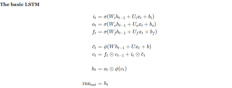
As per the LSTM literature, there are 3 things a LSTM should selectively decide, “what to write, what to read and what to forget”. The most fundamental and mathematical way of maintaining selectivity is gates, we call these gates the read, write and forget gates. Our three gates at time step t are denoted i(t), the input gate (for writing), o(t), the output gate (for reading) and f(t), the forget gate (for remembering!).

Here are the mathematical definitions of the gates (notice the similarities):

Equations governing LSTM.

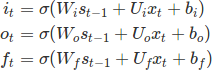
With all the gates defined, we now develop a LSTM prototype by defining the required behavior. To write a candidate state s(t), we follow a simple rule of thumb.

1. Take the inputs using the write gate
2. Calculate the output using the read gate (output is reading the input information so you can remember that it uses the read gate and not the input)
3. Combine the output with relevant prior information, for keeping relevant information we use the forget gate with prior state.

Equations governing LSTM.

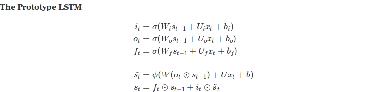
Below is a pictorial view of above equations with arrows pointing to flow of data within the LSTM cell.

A LSTM cell.

In theory, this prototype should work but turns out it doesn’t. It happens because, even after well thought initializations and write and forget gates, the coordination between these gates in early stage of training gets tricky and very often it becomes large and chaotic at write step. For more details, refer to “internal state drift” problem, further, an empirical demonstration of this can be found in Greff et al. (2015), which covers 8 variants of LSTMs.

The solution to above problem is bounding the state to prevent it from becoming chaotic or blowing up. There are 3 variants of LSTM which uses this solution 1. Normalized LSTM, GRU and Pseudo LSTM. We will focus mainly on the GRU for this post but feel free to dive deeper into the other variants.

GRUs

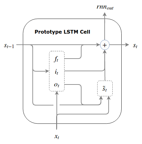
We impose a hard bound on the state by explicitly binding the write and forget gate. In other words, instead of doing selective writes and selective forgets, we define forget as 1 minus write gate. So whatever is not written is forgotten. In the GRU terminology, the forget gate is renamed as update gate or z(t) and it essentially means “do-not-update”. So an element wise update on prior state would tell what not to update and 1 - z(t) actually updates the state behaving as the new write gate.

Equations governing GRU.

Below is a pictorial view of above equations with arrows pointing to flow of data within the GRU cell.

A GRU cell.

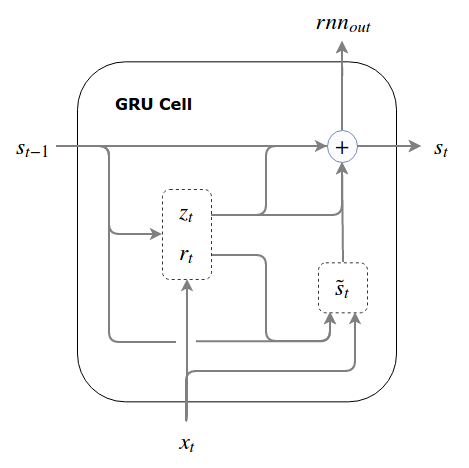
Note the difference between reads and writes: If we choose not to read from a unit, it cannot affect any element of our state and our read decision impacts the entire state. If we choose not to write to a unit, that impacts only that single element of our state. This does not mean the impact of selective reads is more significant than the impact of selective writes: reads are summed together and squashed by a non-linearity, whereas writes are absolute, so that the impact of a read decision is broad but shallow, and the impact of a write decision is narrow but deep.

You might still be wondering that the LSTM cell we talked about doesn’t quiet look like the Basic LSTM cell available all over Internet and you are right. The reason is we didn’t define the Basic LSTM cell above, we defined a prototype cell we sequentially answered all the problems faced with vanilla RNNs. We will now move forward to define the Basic LSTM cell.

Basic LSTM cell

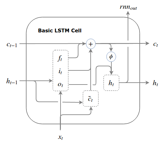
As we discussed above, read comes after write because the cell writes the input to memory and then reads the output during calculation followed by finally applying the forget gate and update the cell. Here we loosely used the term memory which plays an important role in the construct of basic LSTM cell. The Basic LSTM cell requires a small change from our prototype, we will now input 2 priors to a cell, namely, previous state s(t) now renamed as c(t) and a shadow/hidden state h(t). Hidden state is nothing but a gated previous state and additionally the previous also flows in the cell. The output of this a an updated current state along with a hidden state which is a gated current state.

If we think carefully, the basic LSTM is taking the previous state in 2 forms, directly and gated (other than the external input)and producing current state in 2 forms, directly updated ans its gated version. The primary reason of introducing all this complexity and the hidden states is the “write then read order”. We need to read the previous state in order to create a current candidate write. But if, creating the current candidate write, comes before the read operation inside our cell, we can’t do that unless we pass a pre-gated “previous state”, which makes hidden states compulsory. The write-then-read order thus forces the LSTM to pass a hidden state from cell to cell.

Basic LSTM equations updated with respect to the memory cell view.

Below is a pictorial view of above equations with arrows pointing to flow of data within the Basic LSTM cell.

A Basic LSTM cell, as available across Deep Learning Libraries.

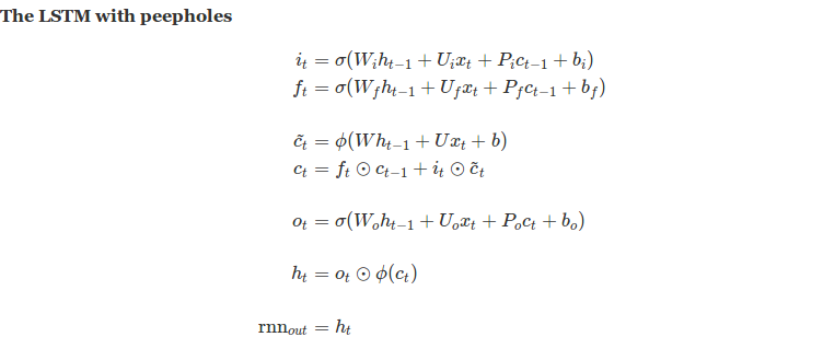
Though this implementation of LSTM is stable and scales well, the unmodified previous state input is sometimes re-wired to flow into the gates calculation giving birth to LSTM with peepholes, which is simply another variant of LSTM. The primary difference with peephole LSTM is that the updated current state is used for output via read gate as opposed to the prior state read by the Basic LSTM cell.

Governing equations of LSTM with peepholes.

Conclusion

LSTM and its variants solved the fundamental (information morphing) and technical (vanishing gradients) problems associated with RNNs and thus gained popularity. The ideology associated with LSTM and its variants also allowed researchers to implement a similar thought process of selectivity while reading and writing information. This ideology paved way for the Residual Networks or ResNet combined with very deep (upto 100s of layers) architecture. This network won the ImageNet 2015 competition.

The content of this post might get confusing with a visual depiction and thanks to deepsystems.ai you can watch the video for a better understanding. Their video and quoted text of this post is inspired by R2RT’s blog post: Written Memories: Understanding, Deriving and Extending the LSTM.

In the next post, we will look at Auto Encoders in detail and also explore their utility in modern architectures.

Thank you for reading, I hope it helped