Review

Last week we talked about a very particular type of NNet called Convolutional Neural Network. We can definitely dive deeper into Conv Nets but the essence of the topology was broadly covered in the previous post. We will revisit the Conv Nets after we have covered all the topologies, as discussed in the previous post.

Week 2

The architecture for this week is Recurrent Neural Network or RNN. The key difference between a RNN and any Feed Forward Normal/Deep Network is the recurrence or cyclic nature of this architecture. It sounds vague in the first go but lets unroll this architecture to understand it better. We will also be discussing two special cases of RNN namely LSTM and GRU in the next post.

Why do we need RNNs? Lets find out.

Lets take a use-case of RNN, Natural Language Processing (NLP), traditional NLP techniques used statistical methods and rule-based approach to define a language model. Language models computes a probability for a sequence of words: P(w1, w2, ….. wn) which is useful in machine translation and word prediction.

These traditional models have 3 major challenges:

1. Probability was usually conditioned over n previous words.
2. An incorrect but necessary Markov assumption.

1. To estimate any probability they had to compute n-grams.

Computation of so many n-grams has HUGE RAM requirements, which gets practically impossible after a point. Also, above models relied on hand engineered linguistic features to deliver state-of-the-art performance.

RNNs solve the above problems by using a simple solution called “statefulness” and “recurrence”. Deep Learning allows RNN to remember or forget things based on few logical values, as we will see later, and perform cyclic operations within the network to achieve better results. Before we start exploring how all this happens, lets first understand a crucial input that goes into RNN, Word Embeddings.

Word Embeddings

Introduced by Bengio, et al. more than a decade ago, these are powerful representation of simple words. For example, the sentence “the cat ate the food” is the input to a language model, now we need to convert this sentence into numbers for the network to process it. The simplest way is to form One-Hot vectors of vocabulary.

One Hot Encoding

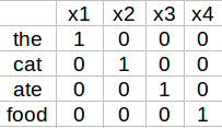
Although this looks simple and gets the job done, think of a scenario where our vocabulary has a Billion words, then we would need 1Bx1B matrix, which is extremely sparse and GIGANTIC in size. To solve this problem, we can develop word embeddings which are dense representation of the word along with its meaning, context, placement in sentence and much more. More technically, word embeddings are a parameterized function mapping in some language to high-dimensionality.

Word Embeddings

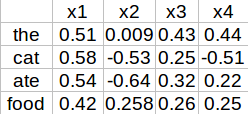
These vectors are dense and allow for more information to be captured for every word, though the meaning of these vectors are a mystery, yet they are more likely to explain a word with better meaning given a large vocabulary set and the dimensionality of these embeddings can be as high as 200 to 500. We can set these embeddings as random and train on our corpus or we can choose transfer learning and utilize pre-trained word representation like Word2Vec and Glove. One thing we can do to understand these embeddings is use a dimensionality reduction technique called t-SNE which helps in visualizing high dimensional data.

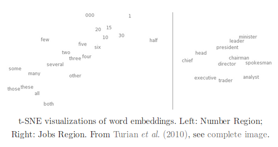
It seems logical for a network to have similar vectors for similar words and if we cluster them after t-SNE the results are fairly intuitive.

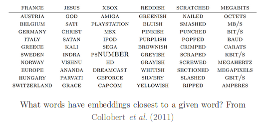
It gets magical when we see analogies encoded as difference in these word vectors, meaning a euclidean distance between words is analogical to their actual meaning set in the language.

Word Embeddings forming analogies.

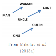
It is safe to assume that if a network is trained over a huge corpus, word embeddings obtained can provide country:language, state/nation:capital, job:role and far more sophisticated relationships. Word embeddings also allow bilingual word connections and entity to image mapping but we will focus on RNNs for this part.

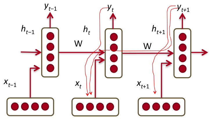
Recurrent Neural Networks

A simple RNN takes a word embedding as input, perform some matrix operations, achieves an interim output called hidden state and then using an activation and previous hidden state it outputs the prediction. Lets assume its a word prediction model and the current output from the model is the most probable word after the first input, so the output for word ‘cat’ should be ‘ate’.

Single layer of RNN.

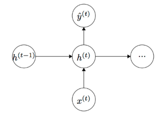
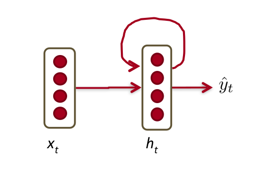
Repeating several such layers makes a RNN recurrent as it visits the information obtained till previous iteration to utilize it in current iteration. There are two ways to look at it, I personally prefer the unfolded depiction of RNNs but people use a cyclic notation as well which seems intuitive.

Unfolded view of RNN.

Cyclic view of RNN.

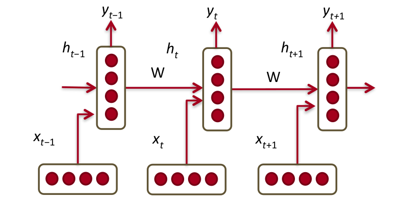
Elaborating on our previous example, the word embedding of cat (lets say we{cat}) takes input from we{the} to predict “ate”, in the next step, we{ate} takes input as combined information from the previous hidden state and account for both we{the} and we{cat} directly to predict “the”. The final iteration will incorporate we{the} with hidden state from previous iteration accounting for we{the}, we{cat}, we{ate} and re-appearance of we{the} to predict “food”. In principle, the network understood the underlying structure of sentence.

Exploding/vanishing gradients

The major problem with RNNs is something called vanishing gradient, since it utilizes the previous hidden state to predict current output, it back-propagates through all hidden states and following the chain rule, the gradients multiply at each iteration finally becoming approximately zero after 7 to 8 words. This doesn’t allow the network to train as expected! Another variant of the same problem is exploding gradient which occurs when the weights of the hidden states are greater than 1, back-propagating leads to infinitely huge values. However there is a simple solution proposed by researchers to avoid exploding gradients which is simply capping the value of gradients to a max. So the only problem we need to deal with is vanishing gradients. Lets welcome the two most popular variant of a RNN, LSTM (Long-Short-Term-Memory) and GRU (Gated Recurrent Unit) networks, we will discuss them in detail in the upcoming post. But before discussing LSTMs and GRUs lets fancy ourselves with Bi-Directional RNNs.

Back propagation leading to vanishing gradients.

Bi-Directional RNNs

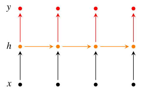
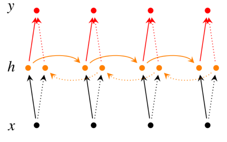
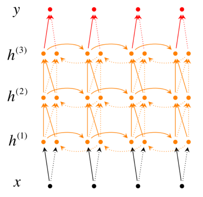
A simple RNN looks like the below diagram, however, if we choose to utilize ‘the next and the previous’ hidden states to predict current output then its called a Bi-Directional RNN. Going ‘deeper’ if we allow more than one hidden layers before our output then its called a Deep Bi-Directional RNN.

A simple RNN in a different view.

A Bi-Directional RNN.

A Deep Bi-Directional RNN.

How does recurrence helps? Is it same as Recursive Neural Networks?

As we discussed above, recurrence is simply using information from previous hidden state which in turn uses previous hidden state so on and so forth. In the “cyclic view” it is easier to understand the “re-occurrence” of referring back to all previous hidden state, which brings the name recurrence. However, we must not confuse it with Recursive Neural Networks which are TREE type RNNS. We can debate that recurrence and recursive indicate the same notion of matrix operations within a network but the structural implementation to utilize this notion of matrix operations to process information sequentially sets them apart. Below example clearly separates the “Recurrent” and “Recursive” neural networks.

Recursive vs. Recurrent Neural Network.

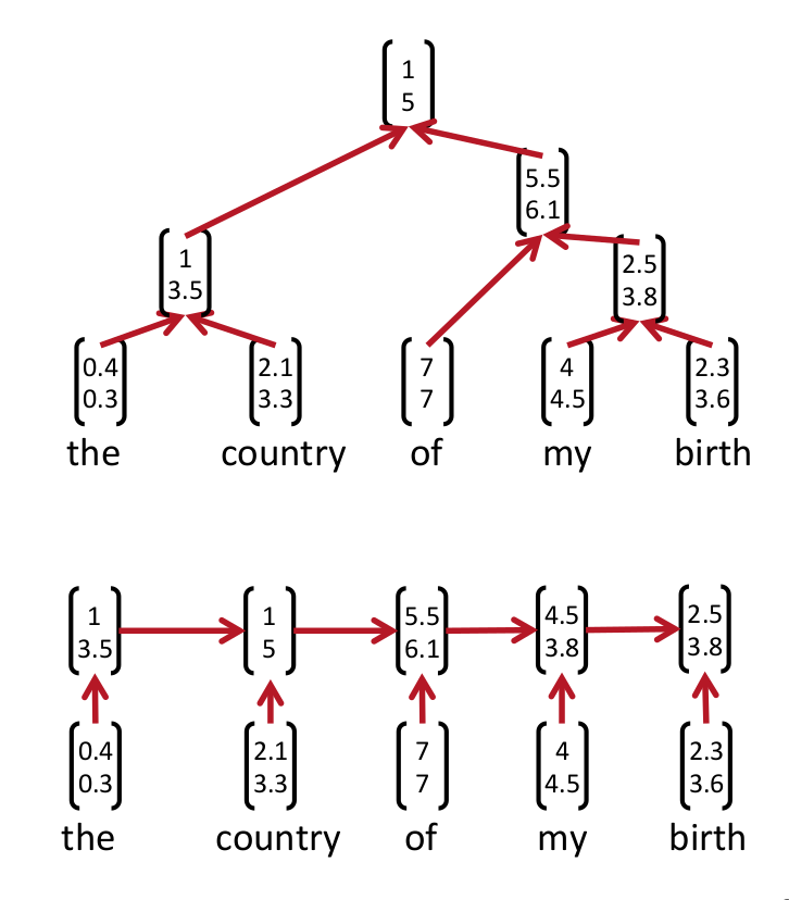
In theory, the recursive NNets require parser to form a tree structure but at the same time, a good parser will allow a tree structure capturing long distance context without a huge bias on the previous word. On the other hand recurrent NNets often capture too much of last word.

Statefulness of RNNs

RNNs can be stateful, which means that they can maintain states during training. As you might have guessed, these states are the hidden states which we saw earlier. The benefits of using stateful RNNs are smaller network sizes and/or lower training times. The disadvantage is that we are now responsible for training the network with a batch size that reflects the periodicity of the data, and resetting the state after each epoch. In addition, data should not be shuffled while training the network, since the order in which the data is presented is relevant for stateful networks.

RNNs by default are trained stateless and we need to explicitly tell the network to maintain states if we wish to use them. We will use this property while discussing LSTMs and GRUs in the next post.

Conclusion

RNNs are powerful NNets not only because they are great at NLP, but in general RNNs dominate in more general purpose tasks. You can read “The Unreasonable Effectiveness of Recurrent Neural Networks” by Andrej Karpathy here. It explains RNNs’ Turing-Complete ability and highlights the benefits of one/many to one/many network representation.

In the next post, we will look at LSTMs and GRUs in detail and also explore few LSTM variants.

Thank you for reading, I hope it helped