Introduction

Deep Learning and AI were the buzz words for 2016; by the mid-2017, they have become more frequent and more confusing. So lets try and understand everything one at a time. We will look into the heart of Deep Learning i.e. Neural Networks (NNets). Most variants of NNets are hard to understand and the underlying architectural components make them all sound (theoretically) and look (graphically) the same.

Thanks to Fjodor van Veen from The Asimov Institute, we have a fair representation of the most popular variants of NNet architectures. Please refer to his blog. To improve our understanding of NNets, we will study and implement one architecture every week. Below are the architectures we will be discussing over the next few weeks.

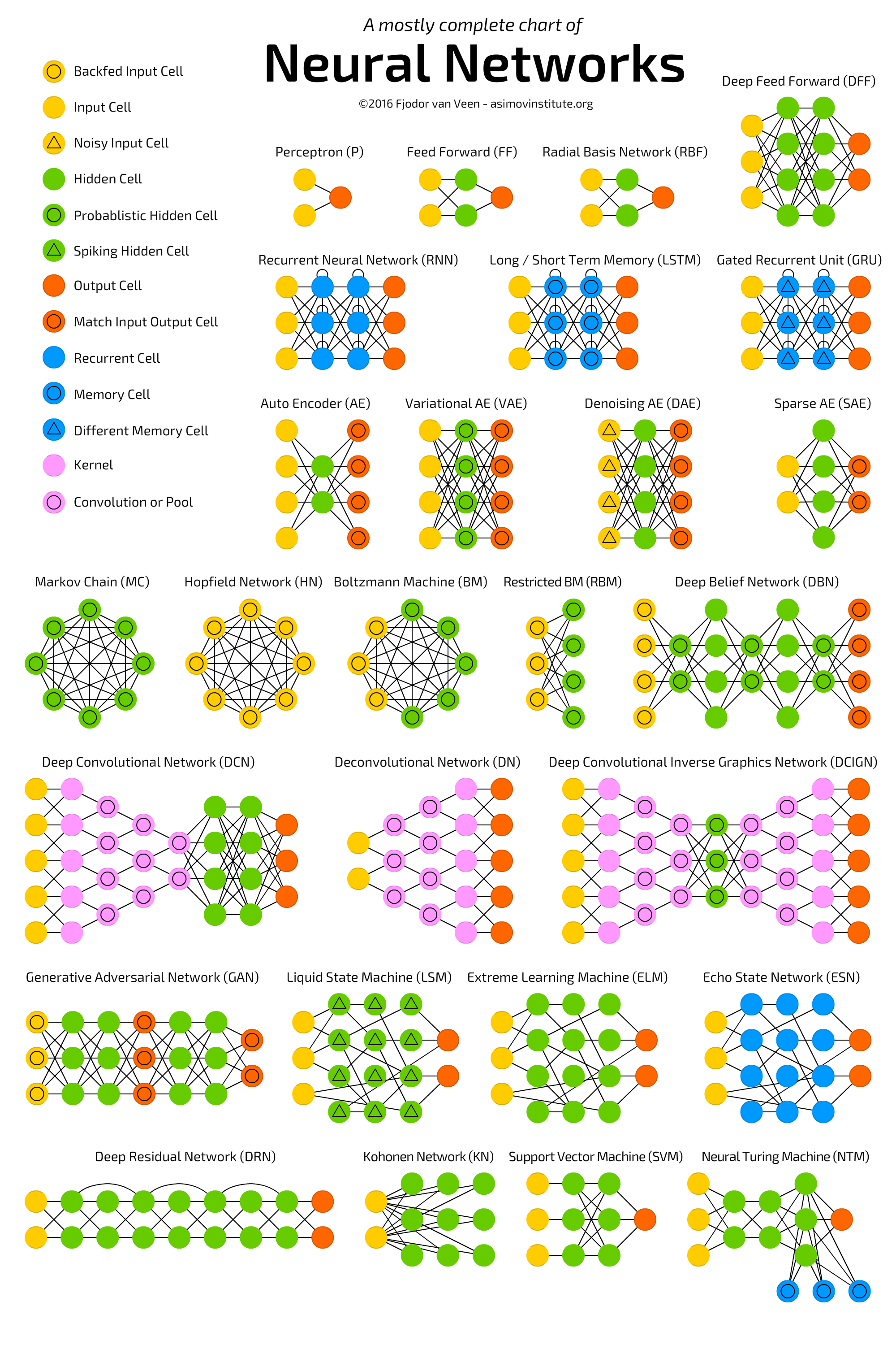
Week 1

The architecture for this week is Convolutional Neural Network or CNN. But before starting CNN, we will first have a small deep dive into Perceptrons. NNet is a collection of several units/cells called perceptrons which are binary linear classifiers. Lets take a quick look to understand the same.

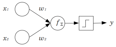
Inputs x1 and x2 are multiplied with their respective weights w1 and w2 and summed together using function f, therefore f = x1*w1 + x2*w2 + b(bias term, optionally added). Now this function f can be any other operation but for perceptrons its generally a summation. This function f is then evaluated through an activation which allows the desired classification. Sigmoid function is the most common activation function used for binary classification. For further details on perceptrons, I recommend this article.

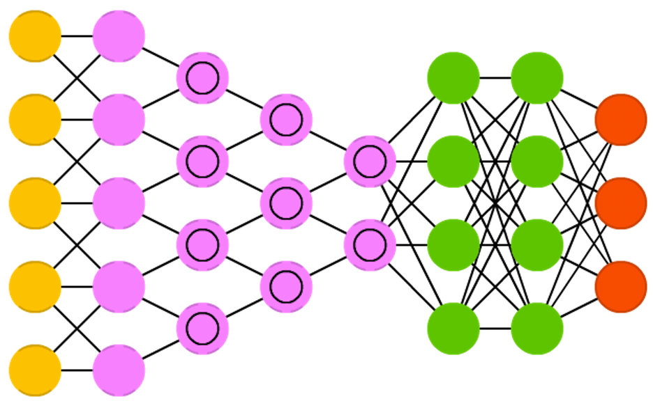
Now if we stack multiple inputs and connect them using function f with multiple cells stacked in another layer, this forms multiple fully connected perceptrons, the output from these cells(Hidden layer) becomes input to the final cell which again uses function f and activation to derive final classification. This, as show below, is the simplest Neural Network.

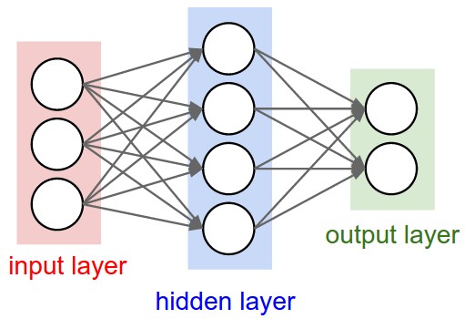
The topologies or architectural variants of NNets are diverse because of a unique capability of NNets called “Universal Approximation function”. This in itself is a huge topic and is best covered by Michael Nielsen here. After reading this we can rely on the fact that NNet can behave as any function no matter how complex. Above mentioned NNets is also referred to as Feed Forward Neural Network or FFNN, since the flow of information is uni-directional and not cyclic. Now that we know the basics of perceptron and FFNN, we can imagine hundreds of inputs connected to several such hidden layer, would form a complex network popular called Deep Neural Network or Deep Feed Forward Network.

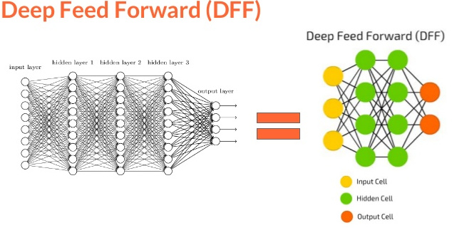
How exactly is a Deep Neural Network different from CNN? Let’s find out.

CNNs gained their popularity through competitions like ImageNet and more recently they are used for NLP and speech recognition as well. A critical point to remember is that many other variants like RNN, LSTM, GRU etc are based on a similar skeleton as that of CNNs but with some difference in architecture that makes them different. We will later discuss the differences in detail.

CNNs are formed using 3 types of layers namely “Convolution”, “Pooling” and “Dense or Fully connected”. Our previous NNets were a typical example of “Dense” layer NNets as all layers were fully connected. To know more about the need to switch to convolution and pooling layers, please read Andrej Karpathy’s excellent explanation here. Continuing our discussion of layers, lets look at convolution layer.

(For the discussion below we will use image classification as a task to understand a CNN, later moving on to NLP and video tasks)

Convolution Layer: Consider an image of 5X5 pixels with 1 as white and o as black, this image is recognized as a monochrome image of dimension 5X5. Now imagine a 3X3 matrix with random 1s and 0s and this matrix is allowed to do a matrix multiplication with a sub-set of image, this multiplication is recorded in a new matrix as our 3X3 matrix moves a pixel in every iteration. Below, is a visual for this process.

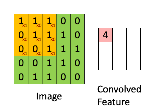
The 3X3 matrix considered above is called a “filter”, which has a task to extract features from the image, it does that by using “Optimization Algorithms” to decide specific 1s and 0s in a 3X3 matrix. We allow several such filters to extract several features in a convolution layer of a NNet. A single step for the 3X3 matrix is called a “stride”

A detailed view of a 3-channel(RGB) image producing two convolution outputs using two 3-channel filters is provided below. Thanks to Andrej Karpathy!

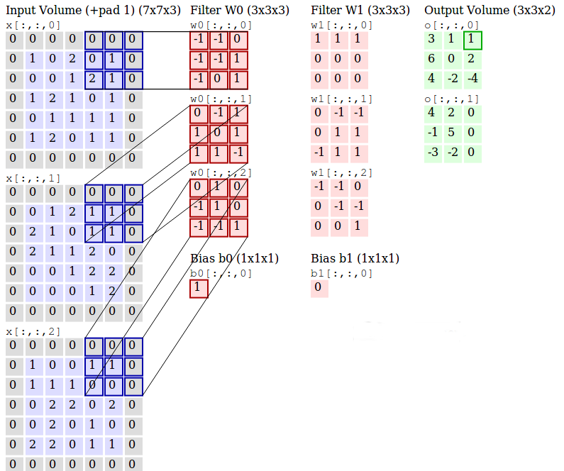
These filters W0 and W1 are the “convolutions” and output is the extracted feature, a layer consisting all these filters is a Convolutional layer.

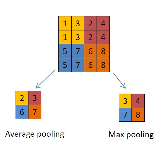
Pooling Layer: This layer is used to reduce the dimension of input using different functions. In general a “MAX Pooling” layer is frequently used after a convolutional layer. Pooling uses a 2X2 matrix and operates over the image in the same manner as a convolution layer but this time its reducing the image itself. Below are 2 ways to pool an image using a “Max Pooling” or “Avg Pooling”

Dense Layer: This layer is a fully connected layer between the activations and the previous layer. This is similar to the simple “Neural Network” we discussed earlier.

Note: Normalization layers are also used in CNN architectures but they will be discussed separately. Also, pooling layers are not preferred since it leads to loss of information. A common practice is to use a larger stride in convolutional layer.

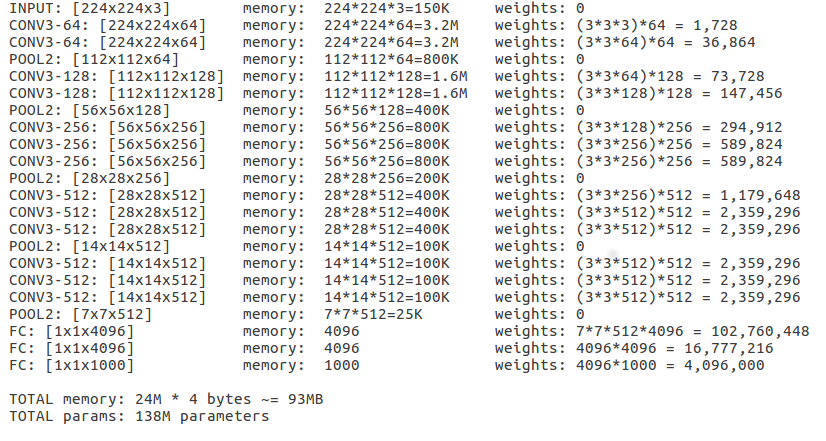
VGGNet, the runner-up in ILSVRC 2014, is a popular CNN and it helped the world to understand the importance of depth in network by using 16 layered network as opposed to 8 layers in AlexNet, ILSVRC 2012 winner. A plug and play model “VGG-16” is available to use in keras, we will be using the same to view a winning CNN architecture.

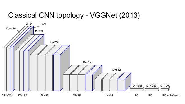
After loading the model in Keras, we can see the “Output Shape” for each layer to understand the tensor dimensions and “Param #” to see how parameters are calculated to obtain the convoluted features. “Param #” is the total weights updates per convoluted feature for all features.

Now that we are familiar with the CNN architectures and understand it’s layers and how it functions, we can move towards understanding how its used in NLP and video processing. This will be covered in the next week’s post along with an introduction to RNNs and the key differences between CNNs and RNNs. Meanwhile, fee free to read about all the CNN models that won ImageNet competitions since 2012, here, Thansk to Adit Deshpande!

Future Work

• Once we have discussed all the architectures, we will follow the same order and implement them using jupyter notebooks. All the code links will be made available once we finish implementation.

• Similar post on updaters
  • ADADELTA
  • ADAGRAD
  • ADAM
  • NESTEROVS
  • NONE
  • RMSPROP
  • SGD
  • CONJUGATE GRADIENT
  • HESSIAN FREE
  • LBFGS
  • LINE GRADIENT DESCENT
• Similar post on Activation functions
  • CUBE
  • ELU
  • HARDSIGMOID
  • HARDTANH
  • IDENTITY
  • LEAKYRELU
  • RATIONALTANH
  • RELU
  • RRELU
  • SIGMOID
  • SOFTMAX
  • SOFTPLUS
  • SOFTSIGN
  • TANH

Thank you for reading, I hope it helped