Review

In the last post we discussed about LSTMs and GRUs, diving deeper into their existence and importance over regular RNNs. Though they are a bit complex, yet they belong to a supervised learning realm which feels intuitive to a large extent when training machine learning models. In next few posts, we will be looking at methods primarily used for deep leaning but with a unsupervised approach.

To start with, we will focus on the benefits of latent representation of data and learning methods to find them. As we discussed earlier in RNNs, embeddings are latent representation of text, similarly, we can find latent representation of images or any other format of unstructured data. But rather than finding a higher dimensional vector representation like embeddings, now we want to focus on learning lower dimensional representation of the data. In this post we will discuss AutoEncoders in great details and set the stage for GANs, RBMs and other NNets which utilize the same concept of information extraction into a lower dimensional space.

AutoEncoders

As the name suggests, AutoEncoders are encoding information without any prior knowledge about the type or distribution of information (technically making them automatic) and hence the name AutoEncoders (AE here on).

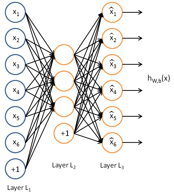
An AE is primarily composed of three parts, an input layer, a hidden layer and a decoding layer. The purpose of this network is to learn the input and recreate it after understanding it! You may come across standard definition saying an AE recreates the input and they are perfectly OK, but then it creates the doubt that is it learning an identity function? meaning is it only replicating the input. Which is not the case and hence the added part to the definition “after understanding it”.

Lets have a close look at the architecture

Autoencoder (Img Src : http://ufldl.stanford.edu)

The AE is trying to learn hW,b(x)≈x, which in essence is equivalent to approximating an identity function but not equal. The difference comes from the design of architecture where we constrain the count of hidden nodes after the input layer. This forces the network to learn weights with which it can still contain the same amount of information but in a lower dimensionality and hence an encoded state which is not an identity state.

However, it is also possible to have higher count of hidden nodes and still find the same amount of information, this is achieved by (as you might have guessed) adding an activation function and limiting the total count of activated nodes to a very low number. This fundamental technique is forcefully introducing sparsity in the network allowing us to achieve the same low dimensional representation. The constant number enforcing the fraction of possible activation is the “sparsity parameter”, now lets dive a little deeper into the math of it.

You can recall that an activation function a(say sigmoid) on an input x gives the output p which is between 0 to 1. This activation acts as a on/off switch for any node in the network (We can achieve the same with tanh as well by defining -1 and 1 as the two states). Now comes the most tricky and fundamental part, if we set the sparsity parameter as p' and define p = a(x), what we are trying to optimize for is p = p'.

Think about it, if the activated output and the sparsity constraints is equal, the output from the activation is 1) densely packed or lower dimensionally encoded (we usually set the sparsity parameter close to 0, for examples 0.05) and 2) it still learned to represent the input x using the network and the activations. So the optimized state directly states “the leaned representation in hidden state is a lower dimensional representation of the input aka the CODE of the AE”. Just to validate our learning, we add a decoding part to the network so that the network can now use the CODE to recreate what it started with and utilize back-propagation to optimize iteratively.

After successfully reducing the loss or finding the best possible CODE, the autoencoder has learned the latent representation of the input data, we can alternatively say, it has learned the distribution of the input data.

NOTE: The optimum state where p' = p is also called the minimum of KL divergence. You can read about it in great details on the web, I suggest this video.

Visualizing an AutoEncoder (Refreshing CNNs)

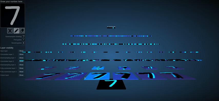
The CODE state of an AE is quite similar to the convolutions learned by a CNN, the difference is, for CNNs the convolutions points to a class(indirectly) and different classes helps build different layers of convolutions as opposed to AEs which try to learn the distribution of the input data so that it can recreate similar new outputs from the learned distribution. For example, the imagenet dataset with 1000 classes help learn edge detection, geometrical shapes, gradients and then faces or more complex/convoluted features from the data, but it only does so to be able to find the boundary condition so that later it can do the classification.

If we look at the rotated view of a CNN forward pass on an image, it looks like a tree with child nodes equal to learned convolutions. While testing an image, it parses the image through this tree structure to gives the highest probability for a class.

NOTE: Fundamentally the encoder half of an AutoEncoder acts as a recognition model and is similar to a CNN, the utilization of the learned representation for AEs and convolutions of CNNs sets them apart.

Tree like view of CNNs

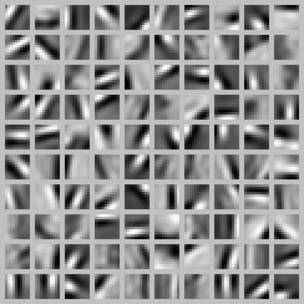
If we look at the CODE for an AE trained on a similar dataset, it looks like an edge detector, but additionally it learned the relative position or better to say, the distribution of the placement of learned edges from the training dataset.

Learned CODE for AutoEncoder

PS: I’m unsure if we can de-couple the convolutions from a CNN and use them as the CODE state with a pre-trained decoder to generate new images/outputs.

Types of AutoEncoders

There are various types of AutoEncoders out there but we will focus on the 4 types clearly mentioned in wikipedia. 1) Denoising AutoEncoder 2) Sparse AutoEncoder 3) Variational AutoEncoder and 4) Contractive AutoEncoder

• Denoising AutoEncoder: The idea is to force the autoencoder to de-noise the data and extract the CODE, to do that, we intentionally add noise with the input data. This technique is an example of good representation which is defined as ‘a representation that can be obtained robustly from a corrupted input and that will be useful for recovering the corresponding clean input’. The only difference while running the code for a denoising autoencoder vs a vanilla autoencoder is passing the noised input rather than the original input and still comparing with the original input.

• Sparse AutoEncoder: We discussed this approach while defining the AutoEncoders.

• Contractive AutoEncoders: They are simply regularized vanilla autoencoders allowing the models to be more robust against slight variations in the input.

• Variational AutoEncoders (VAE): This approach differs in the learning process, a vanilla autoencoder learns the latent representation(CODE) without any prior assumption or belief, whereas VAE assumes that the data is generated by a directed graphical model and that the encoder is learning an approximation to the posterior distribution. I understand that this doesn’t make much sense and for the enormosity and depth of VAE, I will dedicate the next post for a deep dive on VAE and it will also help bring in comparison with GANs. Stay tuned for VAEs…

Conclusion

AutoEncoders are effective way of finding specific latent representation of the training data and there are various implementations and their stacked versions to utilize the best of autoencoders. The encoder is responsible for creating the best patent representation and the decoder is responsible to recreate the input using the learned representation. This makes the decoder half of the AutoEncoder a generative model like GANs. We will look at various generative modeling techniques in the coming posts.

Thank you for reading, I hope it helped